3.5 Confidence Interval for a Parameter
Working through the preceding sections, you may have realized that estimating the value of a statistic in a new sample with a specific precision and probability is not our ultimate goal, as it does not fully represent reality. In reality, we do not know the population parameter, and the primary objective of statistics is to estimate this unknown population parameter.
For example, we don’t care much about the average weight of candies in our sample bag or in the next sample bag that we may buy. We want to say something about the average weight of candies in the population. How can we do this?
In addition, you may have realized that, if we want to construct the sampling distribution of sample means, we first need to know the precise population value, for instance, average candy weight in the population. After all, the average of the sampling distribution is equal to the population mean for an unbiased estimator. In the preceding paragraphs, we acted as if we knew the sampling distribution of sample means.
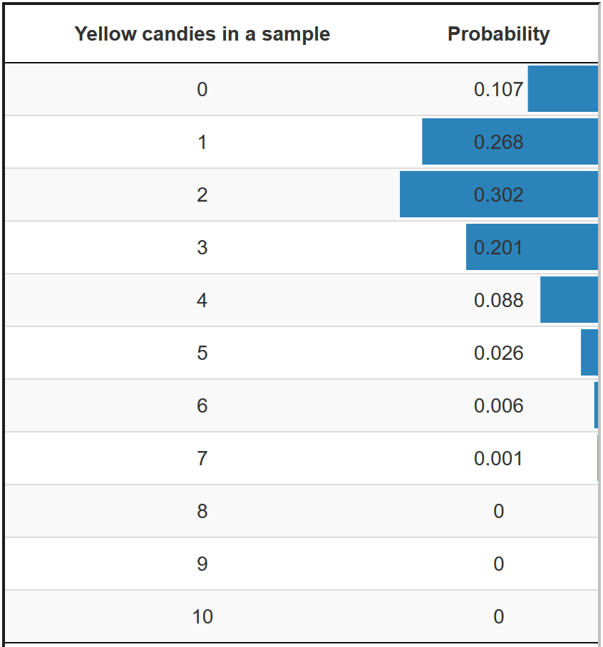
Figure 3.6: Probabilities of a sample with a particular number of yellow candies if 20 per cent of the candies are yellow in the population.
In the exact approach to the sampling distribution of the proportion of yellow candies in a sample bag (Figure 3.6), for instance, we first need to know the proportion of yellow candies in the population. If we know the population proportion, we can calculate the exact probability of getting a sample bag with a particular proportion of yellow candies. But we don’t know the population proportion of yellow candies; we want to estimate it.
In the candy weight example, we first need to know the mean of population candy weight, then we can construct a theoretical probability distribution of sample means. But we do not know the population mean; we want to estimate it.
A theoretical probability distribution can only be used as an approximation of a sampling distribution if we know some characteristics of the population. We know that the sampling distribution of sample means always has the bell shape of a normal distribution or t distribution. However, knowing the shape is not sufficient for using the theoretical distribution as an approximation of the sampling distribution.
We must also know the population mean because it specifies where the centre of the sampling distribution is located. So, we must know the population mean to use a theoretical probability distribution to estimate the population mean.
By the way, we also need the standard error to know how peaked or flat the bell shape is. The standard error can usually be estimated from the data in our sample. But let us not worry about how the standard error is being estimated and focus on estimating the population mean.
3.5.1 Reverse reasoning from one sample mean
In the previous chapters, we were reasoning from population mean to sampling distribution of sample means, then to a single sample mean. Based on the known population mean and standard error, we could draw an interval estimate around the population mean of the sampling distribution (Figure 3.4). 95% of all sample means would fall within this interval estimate around the known population mean.
In practice though, the population mean is unknown. We only have the sample mean derived from our collected data. Using this sample mean, we would like to estimate the population mean.
Figure 3.7: Confidence intervals from replications
Instead of checking whether a sample mean is inside or outside of the interval estimate of the population mean (Chapter 3.4), we use the interval estimate around that one sample mean, to check whether this interval catches the population mean. These two ways are equivalent, but the second way does not require us to know the population mean. This is because the interval estimate around the sample means catches the population mean in 95% of the times, regardless if the population mean is known or not. We call such an interval estimate around the sample mean a 95% confidence interval.
The middle plot of Figure 3.7, shows the 95% confidence interval for a single sample, from the population distribution in the top graph. The green line indicates that the interval estimate around the sample mean catches the population mean. The average candy weight in this samples of \(N=30\) is 2.95 grams and the lower and upper boundary for 95% confidence interval are 2.59 grams and 3.32 grams. We use the blue vertical dashed line to indicate the population mean, which in reality we do not know. Though, in this simulation, we can see that the green 95% confidence interval catches the population mean.
Now, increase the number of times of samples (replications) by adjusting the slider in Figure 3.7. The middle plot now shows how many of the samples with a 95% confidence intervals catch the population mean, indicated by the green lines. The red lines indicate that the 95% confidence interval does not catch the population mean. The percentage that catch the population mean approaches 95% as the number of samples gets higher.
Now, also increase the sample size in Figure 3.7 by moving the slider. We see that, in the middle plot, all confidence intervals become narrower. We therefore are much more confident in our estimation of the population mean with a larger sample size.
Note that the confidence intervals are not of the same with, and that the upper and lower bound for each sample is different. This is because the sample mean is different for each sample, and the standard error is calculated from the sample mean. It is therefore incorrect to say that you are 95% confident that the population mean is within the specific lower and upper bound of your sample. Instead, you are 95% confident that the interval estimate around the sample mean catches the population mean. This is a subtle difference, but indicates that only repeated sampling is the rationale for the confidence that the population mean is within the interval estimate.
If we were to repeat the experiment over and over, then 95% of the time the confidence intervals contain the true mean.
— Hoekstra, Morey, Rouder, & Wagenmakers (2014)
It is very important that we understand that the confidence level 95% is NOT the probability that the population parameter has a particular value, or that it falls within the interval.
In classic statistics (so called “Frequentists”), the population parameter is not a random variable but a fixed, unknown number, which does not have a probability.
A confidence interval around a sample statistics from solely one data collection either catches (100%) or does not catch (0%) the population parameter. We just do not know which one is the case. That’s why we cannot make any conclusion about the population mean based on one confidence interval.
Only when we replicate data collection many many times, we do know that about 95% of all 95% confidence intervals will catch the population mean.Now imagine that you have a large sample for your research project. Looking at Figure 3.7, this would mean that if you would run the same research a hundred times, you would find the population mean within the 95% confidence interval in 95 of these hundred times. That is very reasuring, isn’t it?
In the bottom plot of Figure 3.7, we revisit Chapter 1, to illustrate how these 95% confidence intervals around the sample means are related to the sampling distribution. Each confidence interval in the middle plot is an approximation of the width of the sampling distribution in the bottom plot. The larger the samples size, the narrower the confidence intervals are, and the narrower the sampling distribution becomes in the bottom plot. The histogram represents the sample means from the number replications. Each sample mean comes from one replication.
We also see the theoretical approximation of this sampling distribution (as was discussed in Chapter 2.3) of sample means, which is a normal distribution. As the number of replications and sample size increases, the shape of the histogram gets closer to the shape of the theoretical approximation of the sampling distribution (green line), which in turn also gets narrower.
This sampling distribution is theoretically approximated by a normal distribution whose mean is the population mean and standard deviation is the standard error of the sample. To make our life easier, we can convert the sampling distribution, which is a normal distribution, to the standard normal distribution by converting to a z-score. The critical z value 1.96 and -1.96 together marks the upper and lower limit of the interval containing 95% of all samples with means closest to the population mean.
As a consequence, we are able to calculate 95% confidence interval around a sample mean by adding and subtracting 1.96 standard errors from that sample mean.
- Confidence interval lower limit = sample value – critical value * standard error.
- Confidence interval upper limit = sample value + critical value * standard error.
For example, the 95%-confidence interval for a sample mean:
- Lower limit = sample mean - 1.96 * standard error.
- Upper limit = sample mean + 1.96 * standard error.
Haven’t we seen this calculation before? Yes we did, in Section 3.4.2, where we estimated the interval around population mean for sample means. We now simply reverse the application, using the interval of sample mean to estimate the population mean instead of the other way around.
Jerzy Neyman introduced the concept of a confidence interval in 1937:
“In what follows, we shall consider in full detail the problem of estimation by interval. We shall show that it can be solved entirely on the ground of the theory of probability as adopted in this paper, without appealing to any new principles or measures of uncertainty in our judgements”. (Neyman, 1937: 347)
Photo of Jerzy Neyman by Ohonik, Commons Wikimedia, CC BY-SA 4.0]3.5.2 Confidence intervals with bootstrapping
If we approximate the sampling distribution with a theoretical probability distribution such as the normal (z) or t distribution, critical values and the standard error are used to calculate the confidence interval (see Section 3.5.1).
There are theoretical probability distributions that do not work with a standard error, such as the F distribution or chi-squared distribution. If we use those distributions to approximate the sampling distribution of a continuous sample statistic, for instance, the association between two categorical variables, we cannot use the formula for a confidence interval (Section 3.5.1) because we do not have a standard error. We must use bootstrapping to obtain a confidence interval.
As you might remember from Section 2.5, we simulate a sampling distribution if we bootstrap a statistic, for instance median candy weight in a sample bag. We can use this sampling distribution to construct a confidence interval. For example, we take the values separating the bottom 2.5% and the top 2.5% of all samples in the bootstrapped sampling distribution as the lower and upper limits of the 95% confidence interval. We will encounter the bootstrapping method for confidence intervals around regression coefficient of mediator again in chapter 11.
It is also possible to construct the entire sampling distribution in exact approaches to the sampling distribution. Both the standard error and percentiles can be used to create confidence intervals. This can be very demanding in terms of computer time, so exact approaches to the sampling distribution usually only report p values (see Section 4.2.6), not confidence intervals.