4.1 Hypothesis
The assumption that a researcher wants to test is called a research hypothesis. It is a statement about the empirical world that can be tested against data. Communication scientists, for instance, may hypothesize that:
- a television station reaches half of all households in a country,
- media literacy is below a particular standard (for instance, 5.5 on a 10-point scale) among children,
- opinions about immigrants are not equally polarized among young and old voters,
- the celebrity endorsing a fundraising campaign makes a difference to adult’s willingness to donate,
- more exposure to brand advertisements increases brand awareness among consumers,
- and so on.
These are statements about populations: all households in a country, children, voters, adults, and consumers. As these examples illustrate, research hypotheses seldom refer to statistics such as means, proportions, variances, or correlations. Still, we need a statistic to test a hypothesis. The researcher must translate the research hypothesis into a new hypothesis that refers to a statistic in the population, for example, the population mean. The new hypothesis is called a statistical hypothesis.
A statistical hypothesis is a statement about the empirical world that can be tested against data. It is a statement about the population, not the sample. For example, a hypothesis could be that the average age of a population is 30 years, that the average waight of candy bags is 500 grams, that the proportion of people that like a certain brand is .5, or that the correlation between two variables is .3. These are all statements about the population, not the sample.
Scientists test these hypotheses by following the empirical cycle (de Groot, 1969), which involves a systematic process of induction, deduction, testing, and evaluation. Based on the results, hypotheses can be either rejected or not rejected. If the hypothesis is based on theory and previous research, the scientist uses previous knowledge. As a next step, the researcher tests the hypothesis against data collected for this purpose. If the data contradict the hypothesis, the hypothesis is rejected and the researcher has to improve the theory. If the data does not contradict the hypothesis, it is not rejected and, for the time being, the researcher does not have to change the theory.
Statistical hypotheses usually come in pairs: a null hypothesis (H0) and an alternative hypothesis (H1 / HA). We met the null hypothesis in the preceding sections. We use it to create a (hypothetical) sampling distribution. To this end, a null hypothesis must specify one value for the population statistic that we are interested in, for example, .5 as the proportion of yellow candies.
4.1.1 Null hypothesis
The null hypothesis reflects the skeptical stance in research. It assumes that there is nothing going on. There is no difference between experimental conditions, the new intervention is not better than the previous, there is no correlation between variables, there is no predictive value to your regression model, a coin is fair, and so forth. Equation (4.1) shows some examples of null hypotheses expressed in test statistics.
\[\begin{equation} \begin{split} H_{0} & : \theta & = .5 \\ H_{0} & : \hat{x} & = \mu = 100 \\ H_{0} & : t & = 0 \\ H_{0} & : \mu_1 & = \mu_2 \\ \end{split} \tag{4.1} \end{equation}\]
The null hypothesis does not always assume that the population parameter is zero; it can take any specified value. For instance, a null hypothesis might state that there is no difference in intelligence between communication science students and the general population. In this case, we could compare the average intelligence score of a sample of communication science students to the known population average of 100. Although we are testing whether the difference is zero, in practical terms, we express the null hypothesis as the sample mean being equal to 100.
Though a null hypothesis can be expressed as a single value, that does not mean that we always get that specific value when we take a random sample. Given the null hypothesis that our candy factory machine produces bags with an average of 5 out of 10 yellow candies, there remains a probability that some bags will contain as few as one yellow candy or even none at all. This variability is illustrated in Figure 4.1, which shows that while values near the expected 5 yellow candies are most likely, deviations can occur.
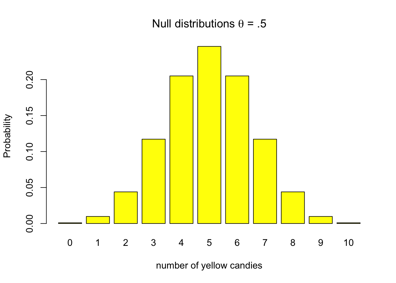
Figure 4.1: Discrete binomial distributions
4.1.2 Alternative hypothesis
The alternative hypothesis indicates what the researcher expects in terms of effects, differences, deviation from null. It is the operationalization of what you expect to find if your theory would be accurate. This would mean that our expected effect of difference would indeed reflect the true population value.
Lets assume for the case of our candy factory example, that the machines parameter is .2. We would expect the machine to produces bags with 2 out of 10 yellow candies, one in five yellow candies per bag. Assuming .2 as the machine’s parameter does not ensure that every bag will contain exactly 2 yellow candies. Some bags will contain 0, 1, 3, 4, 5, 6, 7, 8, 9, or even 10 yellow candies. The probabilities for each can again be visualized using the exact discrete binomial probability distribution (Figure 4.2) as we did for the null hypothesis.
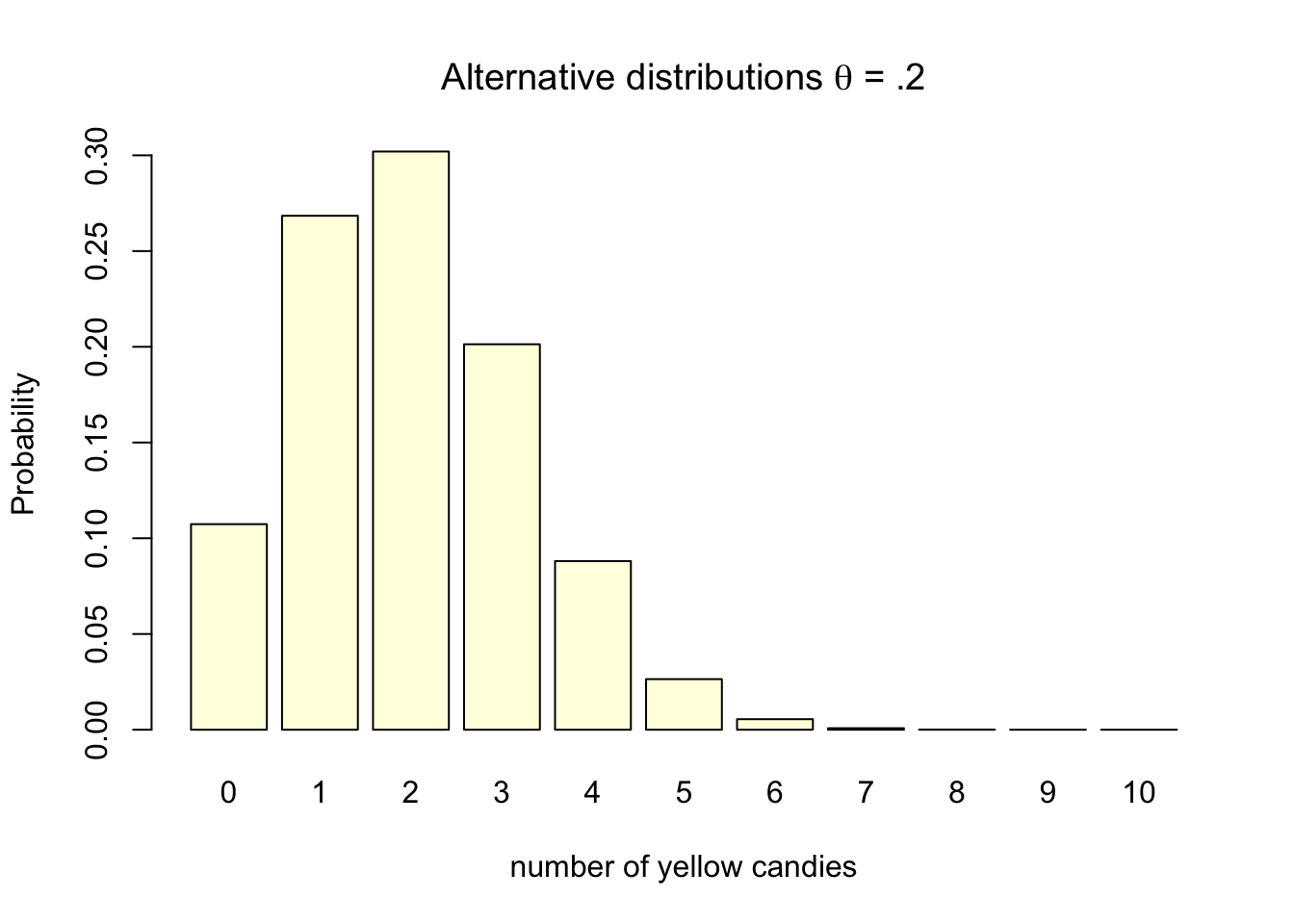
Figure 4.2: Discrete binomial distributions
Note that the probability distribution for \(H_0\) indicates the null assumption about reality, while the probability distribution for \(H_A\) is based on the true population value. At this stage only the sample size, the amount of candies in a bag (10), the null assumption and our knowledge about reality has been used to determine the distribution. No data has been gathered yet in determining these distributions.
When we do research, we do not know the true population value. If we did, no research would be needed of course. What we do have is theories, previous research, and other empirical evidence. Based on this, we can make an educated guess about the true population value. This educated guess is expressed as the alternative hypothesis. The alternative hypothesis is the hypothesis that the researcher expects to find if the theory is accurate. It is the hypothesis that the researcher wants to test using data.
The alternative hypothesis is usually formulated as either not equal to the null hypothesis, or greater than or less than the null hypothesis. Equation (4.2) shows some examples of alternative hypotheses expressed in test statistics.
\[\begin{equation} \begin{split} \text{Two-sided} \\ H_{A} & : \theta & \neq .5 \\ H_{A} & : \hat{x} & \neq \mu \\ H_{A} & : t & \neq 0 \\ H_{A} & : \mu_1 & \neq \mu_2 \\ \text{One-sided} \\ H_{A} & : \theta & < .5 \\ H_{A} & : \hat{x} & > 100 \\ H_{A} & : t & > 0 \\ H_{A} & : \mu_1 & < \mu_2 \\ \end{split} \tag{4.2} \end{equation}\]
The alternative hypothesis can be one-sided or two-sided. A two-sided alternative hypothesis states that the population value is not equal to the null hypothesis. A one-sided alternative hypothesis states that the population value is either greater than or less than the null hypothesis. The choice between a one-sided and two-sided test depends on the research question and the theory. We will cover one and two-sided testing more extensively in Chapter 4.2.12.
4.1.3 Testing hypothesis
In the empirical cycle, the researcher tests the hypothesis against data collected for this purpose. The most widely used method for testing hypotheses is null hypothesis significance testing (NHST). As we will read in this chapter, there are other methods that can be used to test hypotheses, such as confidence intervals and Bayesian statistics.
All methods serve as decision frameworks that enable researchers to establish rules for evaluating their hypotheses. These rules are determined before data collection and are designed to minimize the risk of incorrect decisions. Null Hypothesis Significance Testing (NHST) manages this risk by defining it probabilistically. Confidence intervals provide a measure of accuracy through their width, while Bayesian statistics express this risk in terms of the credibility interval.
In the next chapters, we will cover the logic behind NHST, confidence intervals, and Bayesian statistics. We will also discuss how to select the appropriate statistical test for your research question, and how to report the results of your statistical tests.