6.3 Different Lines for Different Groups
What if the effect of campaign exposure on attitude towards smoking may be different in different contexts, e.g., for people who smoke themselves and people who do not smoke? Perhaps, the campaign is more effective among smokers than among non-smokers or the other way around. If so, the effect of campaign exposure is moderated by the smoking status of the participants.
In a conceptual diagram (Figure 6.14), moderation is represented by an arrow pointing at another arrow. The moderator (smoking status) changes the relation between the predictor (campaign exposure) and the dependent variable (attitude towards smoking).
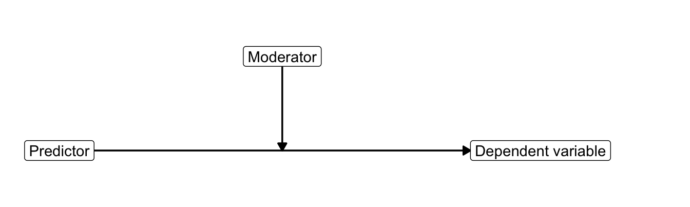
Figure 6.14: Conceptual diagram of moderation.
We used a similar diagram to express moderation in two-way analysis of variance (Section 5.4). But now at least one of our independent variables is numeric, for example, the number of times the respondent has been exposed to the campaign.
Analysis of variance (ANOVA) investigates the effects of categorical variables on a numerical dependent variable. It cannot handle numerical independent variables. Although there are ways to include numerical independent variables in analysis of variance, for example, analysis of covariance (ANCOVA), we use regression analysis if we have a numerical dependent variable and at least one numerical independent variable.
In the current section, we discuss regression models with a numerical predictor and a categorical moderator. The next chapter (Chapter 7) presents regression models in which both the predictor and the moderator are numerical.
6.3.1 A dichotomous moderator and numerical predictor
Figure 6.15: Is the effect of exposure on attitude moderated by smoking status?
In Section 6.1, we have analyzed the predictive effects of exposure to an anti-smoking campaign and smoking status on a person’s attitude towards smoking. We have found a negative effect for exposure and a positive effect for smoking. More exposure predicts a more negative attitude whereas smokers have on average a more positive attitude towards smoking than non-smokers.
Our current question is: Does exposure to the campaign have the same effect for smokers and non-smokers? We want to compare an effect (exposure on attitude) for different contexts (smokers versus non-smokers), so our current question involves moderation. Is the effect of exposure on attitude moderated by smoking status?
Our moderator (smoker vs. non-smoker) is a dichotomous variable but our predictor (exposure) is numerical, so we cannot use analysis of variance. Instead, we use regression analysis, which allows numerical predictors.
In the context of a regression model, moderation means different slopes for different groups. The slope of the regression line is the regression coefficient, which expresses the effect of the predictor on the dependent variable. If we have different effects in different contexts (moderation), we must have different regression coefficients for different groups.
6.3.2 Interaction variable
How do we obtain different regression coefficients and lines for smokers and non-smokers? The statistical trick is quite easy: Include an additional predictor in the model that is the product of the predictor (exposure) and the moderator (smoking status). This new predictor is the interaction variable. The regression coefficient of the interaction variable is called the interaction effect.
Figure 6.16: How does an interaction variable create different regression lines for different groups?
The interaction variable must be included together with the original predictor and moderator variables, see Equation (6.12). This is also visible in the statistical diagram (Figure 6.17) for moderation in a regression model.
\[\begin{equation} \small \begin{split} attitude = &\ constant + b_1*exposure + b_2*smoker + b_3*exposure*smoker \end{split} \tag{6.12} \normalsize \end{equation}\]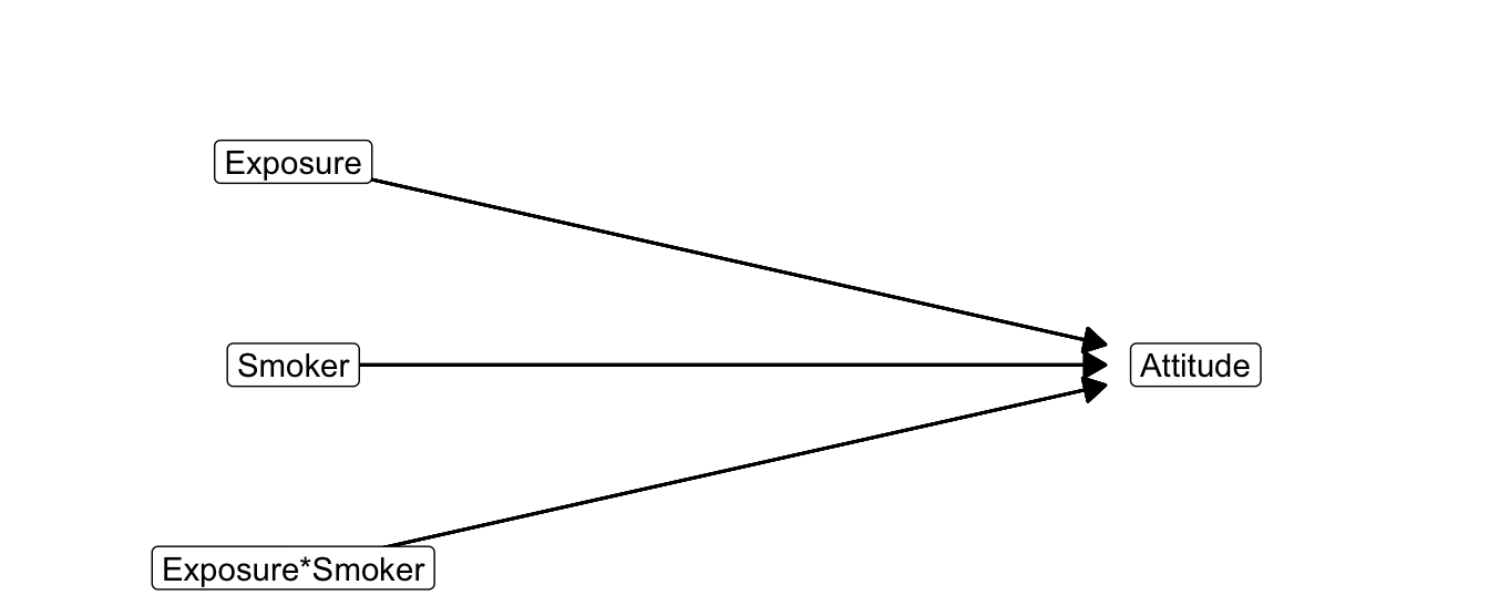
Figure 6.17: Statistical diagram of moderation.
The smoking status variable is coded 1 for smokers and 0 for non-smokers. For clarity, we name this variable smoker with score 1 for Yes and score 0 for No. We have two different regression equations, one for each group on the dichotomous predictor smoker. Just plug in the two possible values (1 and 0) for this variable. For non-smokers [Equation (6.13)], the interaction variable drops from the model because multiplying by zero yields zero. For non-smokers, our reference group, \(b_1\) represents the effect of exposure on attitude. It is called the simple slope of exposure for non-smokers.
\[\begin{equation} \small \begin{split} attitude = &\ constant + b_1*exposure + b_2*smoker + b_3*exposure*smoker \\ attitude_{non-smokers} = &\ constant + b_1*exposure + b_2*0 + b_3*exposure*0 \\ attitude_{non-smokers} = &\ constant + b_1*exposure \end{split} \tag{6.13} \normalsize \end{equation}\]In contrast, the interaction variable remains in the model for smokers [Equation (6.14)], who score 1 on smoking status. Note what happens with the coefficient of the exposure effect if we rearrange the terms a little: The exposure effect equals the effect for the reference group of non-smokers (\(b_1\)) plus the effect of the interaction variable (\(b_3\)). The simple slope for smokers, then, is (\(b_1 + b_3\)).
\[\begin{equation} \small \begin{split} attitude = &\ constant + b_1*exposure + b_2*smoker + b_3*exposure*smoker \\ attitude_{smokers} = &\ constant + b_1*exposure + b_2*1 + b_3*exposure*1 \\ attitude_{smokers} = &\ constant + b_1*exposure + b_3*exposure + b_2 \\ attitude_{smokers} = &\ constant + (b_1 + b_3)*exposure + b_2 \end{split} \tag{6.14} \normalsize \end{equation}\]The interaction variable changes the slope of the effect of exposure on attitude. More specifically, the regression coefficient of the interaction variable (\(b_3\)) shows the difference between the simple slope of the exposure effect for smokers (\(b_1+b_3\)) and the simple slope for non-smokers (\(b_1\)).
Let us assume that the unstandardized regression coefficient of the interaction effect is -0.3. This means that the effect of exposure on attitude is more strongly negative (or less positive) for smokers than for non-smokers. One additional unit of exposure decreases the predicted attitude for smokers by 0.3 more than for non-smokers.
6.3.3 Conditional effects, not main effects
It is very important to note that the effects of exposure and smoking status in a model with exposure by smoking status interaction are not main effects as in analysis of variance. As we have seen in the preceding section [Equation (6.13)], the regression coefficient \(b_1\) for exposure expresses the effect of exposure for non-smokers. It is a conditional effect, namely the effect for non-smokers only. Non-smokers are the reference group because they score zero on the moderator (smoker). This is quite different from a main effect in analysis of variance, which is an average effect over all groups.
In a similar way, the regression coefficient \(b_2\) for smoking status expresses the effect for persons who score zero on the exposure predictor. Simply plug in the value 0 for exposure in the regression equation [Eq. (6.15)].
\[\begin{equation} \small \begin{split} attitude = &\ constant + b_1*exposure + b_2*smoker + b_3*exposure*smoker\\ attitude_{no-expo} = &\ constant + b_1*0 + b_2*smoker + b_3*0*smoker \\ attitude_{no-expo} = &\ constant + b_2*smoker \end{split} \tag{6.15} \normalsize \end{equation}\]Smoking status is a dichotomy, so its regression coefficient (\(b_2\)) tells us the average difference in attitude between smokers and non-smokers. Due to the inclusion of the interaction variable, it now tells us the difference in average attitude between smokers and non-smokers who have zero exposure to the anti-smoking campaign. Note again that this is a conditional effect, not a main effect.
6.3.4 Interpretation and statistical inference
| B | Std. Error | Beta | t | Sig. | Lower Bound | Upper Bound | |
|---|---|---|---|---|---|---|---|
| (Constant) | 0.900 | 0.357 | 2.521 | 0.014 | 0.190 | 1.610 | |
| Exposure | -0.162 | 0.061 | -0.410 | -2.651 | 0.010 | -0.284 | -0.040 |
| Status (smoker = 1, non-smoker = 0) | 1.980 | 0.738 | 0.096 | 2.683 | 0.009 | 0.512 | 3.448 |
| Exposure*Status (smoker) | -0.327 | 0.142 | -0.238 | -2.311 | 0.023 | -0.609 | -0.045 |
In Table 6.2, the effect of exposure on attitude depends on the value of smoking status because the model includes an interaction effect of exposure with smoking status (red). Non-smokers are the reference group on the smoking status dummy variable because they are coded 0. Therefore, the regression coefficient for exposure (blue) gives us the effect of exposure on smoking attitude for non-smokers. If you want to check this, plug in 0 for the smoking status variable in the regression equation that we may construct from Table 6.2.
\[\begin{equation} \small \begin{split} attitude = &\ \color{#FDAE61}{constant} + \color{#2B83BA}{b_1*exposure} + \color{#ABDDA4}{b_2*status} + \color{#D7191C}{b_3*exposure*status}\\ attitude_{non-smoker} = &\ \color{#FDAE61}{0.900} + \color{#2B83BA}{-0.162*exposure} + \color{#ABDDA4}{1.980*0} + \color{#D7191C}{-0.327*exposure*0}\\ attitude_{non-smoker} = &\ \color{#FDAE61}{0.900} + \color{#2B83BA}{-0.162*exposure} + \color{#ABDDA4}{0} + \color{#D7191C}{0}\\ attitude_{non-smoker} = &\ \color{#FDAE61}{0.900} + \color{#2B83BA}{-0.162*exposure} \end{split} \tag{6.16} \normalsize \end{equation}\]Multiplying by zero yields zero, so for non-smokers, the resulting effect of exposure on attitude is -0.16. An additional unit of exposure predicts a smoking attitude among non-smokers that is 0.16 points more negative. More exposure to the campaign goes together with a more negative attitude towards smoking for non-smokers. The p value for this effect tests the null hypothesis that the effect is zero in the population. If the exposure effect is statistically significant, we reject this null hypothesis.
Smokers are coded 1 on the (smoking) status variable and non-smokers are coded 0, so the regression coefficient for the interaction variable tells us that the slope of the exposure effect is 0.33 lower for smokers than for non-smokers. The estimated slope of the exposure effect is -0.16 for non-smokers. We can add the regression coefficient of the interaction variable to obtain the estimated slope for smokers, which is -0.49.
If you want to check this, plug in 1 for the smoking status variable in the regression equation. Add the two effects of exposure in the equation to obtain the effect of exposure on attitude for smokers.
\[\begin{equation} \small \begin{split} attitude = &\ \color{#FDAE61}{constant} + \color{#2B83BA}{b_1*exposure} + \color{#ABDDA4}{b_2*status} + \color{#D7191C}{b_3*exposure*status}\\ attitude_{smoker} = &\ \color{#FDAE61}{0.900} + \color{#2B83BA}{-0.162*exposure} + \color{#ABDDA4}{1.980*1} + \color{#D7191C}{-0.327*exposure*1}\\ attitude_{smoker} = &\ \color{#FDAE61}{0.900} + \color{#2B83BA}{-0.162*exposure} + \color{#ABDDA4}{1.980} + \color{#D7191C}{-0.327*exposure}\\ attitude_{smoker} = &\ \color{#FDAE61}{0.900} + \color{#2B83BA}{-0.162*exposure} + \color{#D7191C}{-0.327*exposure} + \color{#ABDDA4}{1.980}\\ attitude_{smoker} = &\ \color{#FDAE61}{0.900} + (\color{#2B83BA}{-0.162} + \color{#D7191C}{-0.327})*exposure + \color{#ABDDA4}{1.980}\\ attitude_{smoker} = &\ \color{#FDAE61}{0.900} + -0.489*exposure + \color{#ABDDA4}{1.980} \end{split} \tag{6.17} \normalsize \end{equation}\]Now we can compare the slopes (regression coefficients) for the two groups, which gives good insight into the nature of moderation in this example. The effect of exposure on attitude is more strongly negative for smokers (-0.49) than for non-smokers (-0.16).
The interaction variable is treated as an ordinary predictor in the estimation process, so it receives a confidence interval and a p value. The null hypothesis for the p value is that the interaction effect is zero in the population. In other words, the effect of exposure on attitude is hypothesized to be the same for smokers and non-smokers in the population; no moderation is expected in the population.
We know the confidence intervals and p values of the exposure effect for non-smokers (the regression coefficient for exposure) and for the difference between their exposure effect and the exposure effect for smokers (the regression coefficient for the interaction effect). We do not know, however, the confidence interval and statistical significance of the exposure effect for smokers. We cannot add confidence intervals or p values, so we do not know if the effect of exposure for smokers is significantly different from zero in the population.
If you want to know the confidence interval or p value of the exposure effect for smokers, you have to rerun the regression analysis using a different dummy variable for the moderator. You should create a dichotomous variable that assigns 0 to smokers and 1 to non-smokers, and an interaction variable created with this dichotomy. The regression coefficient of the exposure effect now expresses the effect for smokers because smokers are the reference group on the new dummy variable. The associated p value and confidence interval apply to the exposure effect for smokers.
Interaction variables are used just like ordinary predictors, so the general assumptions of regression analysis apply. See Section 6.1.4 for a description of the assumptions and checks.
In a similar way, the effect of smoking status on attitude is conditional on exposure because smoking status and exposure are included in the interaction variable. The regression coefficient for status tells us the difference between smokers and non-smokers who have 0 exposure. So, without exposure to the campaign, smokers are on average 1.98 more positive towards smoking than non-smokers. The p value tests the null hypothesis that the difference is zero for people without exposure (exposure = 0) to the anti-smoking campaign.
Let us conclude the interpretation with a warning. The standardized regression coefficients that SPSS reports for interaction effects or effects of predictors that are involved in interaction effects must not be used. They are calculated in the wrong way if the regression model includes an interaction variable. As a result, they are misleading.
6.3.5 A categorical moderator
What if we have three or more groups on our moderator? For example, smoking status measured with three categories: (1) never smoked, (2) formerly smoked, (3) currently smoking? Does the effect of exposure on attitude vary between non-smokers, participants who stopped smoking, and those who are still smoking?
Figure 6.18: When do we have moderation with a categorical moderator?
In Section 6.1.3, we learned that we must create dummy variables for all but one groups of a categorical predictor in a regression model. This is what we have to do also for a categorical moderator. If the effect of a predictor, such as exposure, is moderated by a categorical variable, we have to create an interaction variable for each dummy variable in the equation. To create the interaction variables, we multiply the predictor by each of the dummy variables.
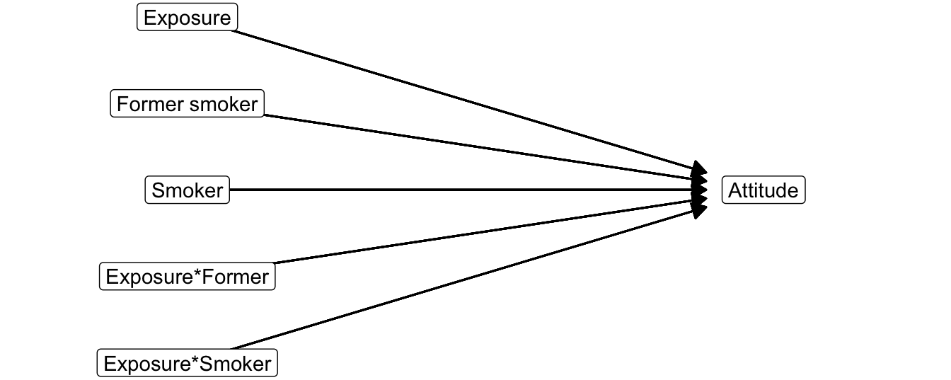
Figure 6.19: Statistical diagram with a moderator consisting of three groups. Non-smokers are the reference group
In the end, we have an interaction variable for all groups but one on the categorical moderator. Figure 6.19 shows the statistical diagram. Estimation of the model yields point estimates (regression coefficients), confidence intervals, and p values for all independent variables (Table 6.3).
| B | Std. Error | t | Sig. | Lower Bound | Upper Bound | |
|---|---|---|---|---|---|---|
| (Constant) | 1.644 | 0.288 | 5.717 | 0.000 | 1.072 | 2.216 |
| Exposure | -0.185 | 0.046 | -3.987 | 0.000 | -0.277 | -0.093 |
| Former smoker | -1.095 | 0.544 | -2.013 | 0.048 | -2.178 | -0.012 |
| Smoker | 1.235 | 0.521 | 2.372 | 0.020 | 0.199 | 2.272 |
| Exposure*Former smoker | -0.405 | 0.112 | -3.604 | 0.001 | -0.629 | -0.181 |
| Exposure*Smoker | -0.304 | 0.098 | -3.116 | 0.003 | -0.498 | -0.110 |
Remember that the effects of predictors that are included in interactions are conditional effects: effects for the reference group or reference value on the other variable involved in the interaction. Non-smokers are the reference group for participant’s smoking status. The p value for the exposure predictor tests the hypothesis that the exposure effect for non-smokers is zero in the population.
For the two dummy variables Former smoker and Smoker, the null hypothesis is tested that they have the same average attitude in the population as the non-smokers (reference group) if they are not exposed to the anti-smoking campaign. Participants who are not exposed to the campaign (zero exposure) are the reference group here.
Interaction predictors show effect differences. In Table 6.3, the interaction predictors test the null hypotheses that the effect of exposure on attitude is equal for former smokers and non-smokers (Exposure*Former smoker) or for smokers and non-smokers (Exposure*Smoker) in the population.
If we would like to know whether the exposure effect for former smokers is significantly different from zero, we have to rerun the regression model using former smokers as reference group. This new model would also tell us whether the exposure effect for former smokers is significantly different from the exposure effect for people who are still smoking.
6.3.6 Common support
In a regression model with moderation, we have to interpret the effect of a predictor involved in an interaction at a particular value of the moderator (Section 6.3.3). The estimated effect at a particular value of the moderator can only be trusted if there are quite some observations at or near this value of the moderator. In addition, these observations should cover the full range of values on the predictor. After all, the effect that we estimate must tell us whether high values on the predictor go together with higher (or lower) values on the dependent variable than low values on the predictor.
For example, we need quite some observations for smokers to estimate the conditional effect of exposure on attitude for smokers. If there are hardly any smokers in our sample, we cannot estimate the effect of exposure on attitude for them in a reliable way. Even if we have quite some observations for smokers but all smokers have low exposure, we cannot say much about the effect of exposure on attitude for them. If we cannot say much about the effect within this group, we cannot say much about the difference between this effect and effects for other groups. In short, the moderation model is problematic in this situation.
Figure 6.20: How well do the observations cover the predictor within each category of smoking status?
The variation of predictor scores for a particular value of the moderator is called common support (Hainmueller, Mummolo, & Xu, 2016). If common support for predictors involved in moderation is poor, we should hesitate to draw conclusions from the estimated effects. Guidelines for good common support are hard to give. Common support is usually acceptable if there are observations over the entire range of the predictor.
It is recommended to check the number of observations per value of the moderator. For a categorical moderator, such as smoking status, a scatter plot of the dependent variable (vertical axis) by predictor (horizontal axis) with dots coloured according to the moderator category may do the job. The left panel of Figure 6.20 shows an example. Check that there are observations for more or less all values of the predictor in each color. If the scatter plot is hard to read, create a histogram of predictor values grouped by moderator categories, as in the right panel of Figure 6.20.
6.3.7 Visualizing moderation and covariates
A plot with different regression lines for different categories of the moderator is a very useful way of presenting your results. We can, however, only plot a regression line if we have a single independent variable. After all, we only have one horizontal (X) axis in a plot to display a predictor.
In a moderation model, we have at least two independent variables: the predictor and the moderator. For example, exposure is our predictor because our interest focuses on the effect of campaign exposure on attitude. Participant’s smoking status is the moderator because we expect different exposure effects for participants with different smoking statuses. We may even have additional independent variables for which we want to control (more on this in Chapter 8), for example, a participant’s contacts with smokers. Let us call these additional independent variables covariates.
A predictor is the independent variable that is currently central to our analysis.
A moderator is an independent variable for which we expect different effects of the predictor.
A covariate is an independent variable that is currently not central to our analysis.Note that the distinction between predictor, moderator, and covariate is temporary. As soon as we focus on another variable, that variable becomes the predictor and the other predictors become moderators or covariates. The distinction between predictor, moderator, and covariate is just terminology to show on which variable we focus.
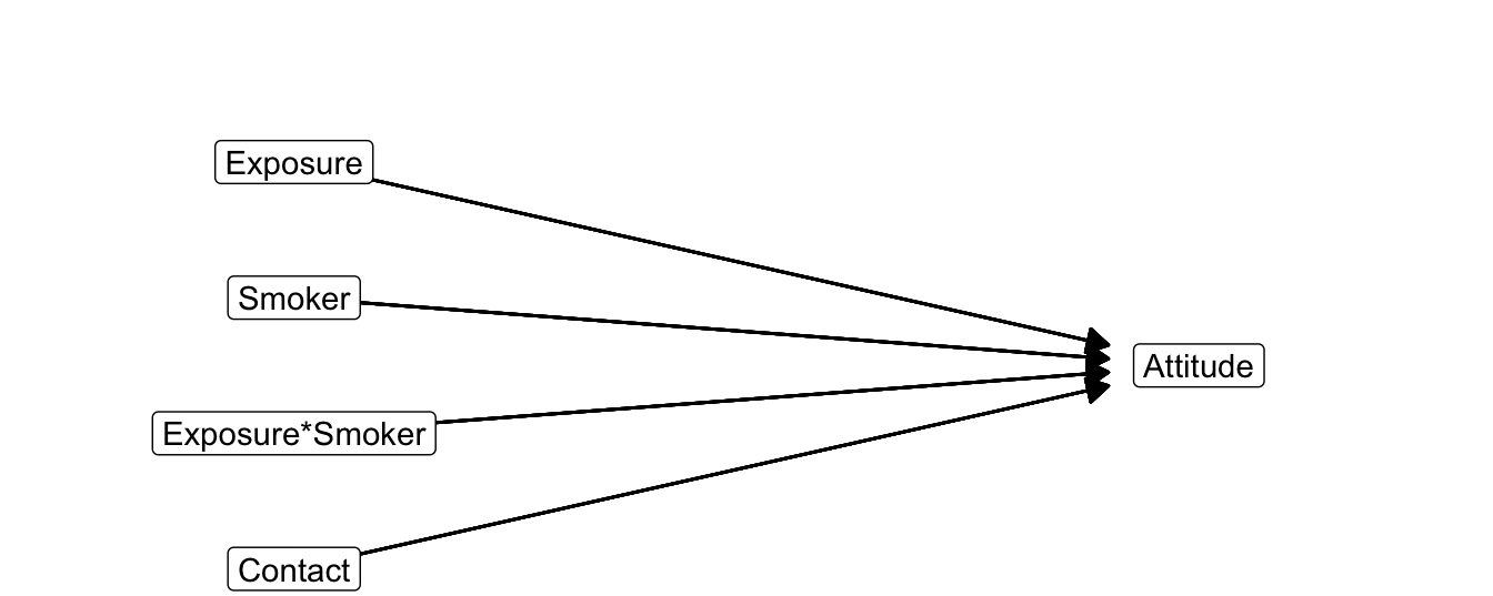
Figure 6.21: Statistical diagram of moderation with contact as covariate.
Figure 6.21 shows the statistical diagram of a moderation model with contact as covariate and Table 6.4 summarizes the estimated effects. How can we get rid of the moderator and covariate(s), so exposure is left as the only independent variable and we can plot regression lines for exposure effects?
| B | Std. Error | Beta | t | Sig. | Lower Bound | Upper Bound | |
|---|---|---|---|---|---|---|---|
| (Constant) | -0.087 | 0.684 | -0.127 | 0.899 | -1.448 | 1.275 | |
| Exposure | -0.118 | 0.066 | -0.332 | -1.786 | 0.078 | -0.249 | 0.013 |
| Smoker (0 = no, 1 = yes)) | 1.982 | 0.730 | 0.095 | 2.717 | 0.008 | 0.530 | 3.434 |
| Exposure*Smoker | -0.329 | 0.140 | -0.239 | -2.348 | 0.021 | -0.607 | -0.050 |
| Contact | 0.152 | 0.090 | 0.180 | 1.683 | 0.096 | -0.028 | 0.331 |
As a first step, use the estimated values of the regression coefficients in the SPSS output (Table 6.4) to create a regression equation [Eq. (6.18)]. Just start at the top of the table and write down the regression coefficients (B) and the independent variable names.
\[\begin{equation} \small \begin{split} attitude = &\ \color{#FDAE61}{-0.087} + \color{#2B83BA}{-0.118*exposure} + \color{#ABDDA4}{1.982*smoker} + \color{#D7191C}{-0.329*exposure*smoker}\\ &+ \color{brown}{0.152*contact} \end{split} \tag{6.18} \normalsize \end{equation}\]As a second step, choose an interesting value for every independent variable in the equation except the predictor. If we want to have the regression line for smokers, choose 1 for the smoker variable. For a numerical covariate such as contact, it is recommended to choose the mean. Average contact with smokers happens to be 5.091 in our example. Now replace the independent variables in the equation by the selected values and simplify the equation [Eq. (6.19)].
\[\begin{equation} \small \begin{split} attitude = &\ \color{#FDAE61}{-0.087} + \color{#2B83BA}{-0.118*exposure} + \color{#ABDDA4}{1.982*smoker} + \color{#D7191C}{-0.329*exposure*smoker}\\ &+ \color{brown}{0.152*contact}\\ attitude = &\ \color{#FDAE61}{-0.087} + \color{#2B83BA}{-0.118*exposure} + \color{#ABDDA4}{1.982*1} + \color{#D7191C}{-0.329*exposure*1} + \color{brown}{0.152*5.091}\\ attitude = &\ \color{#FDAE61}{-0.087} + \color{#2B83BA}{-0.118*exposure} + \color{#ABDDA4}{1.982} + \color{#D7191C}{-0.329*exposure} + \color{brown}{0.772}\\ attitude = &\ (\color{#FDAE61}{-0.087} + \color{#ABDDA4}{1.982}+ \color{brown}{0.772}) + (\color{#2B83BA}{-0.118*exposure} + \color{#D7191C}{-0.329*exposure})\\ attitude = &\ 2.669 + -0.447*exposure \end{split} \tag{6.19} \normalsize \end{equation}\]The terms with smoker and contact disappear from the equation, so exposure is the only independent variable that remains in the equation. Now, we can draw the simple regression line predicting attitude from exposure for smokers using this equation. Note that this is the regression line for people with average contact with smokers.
Repeat these steps but plug in the score 0 for the smoker predictor to obtain the simple regression line for non-smokers. Figure 6.22 shows the two regression lines and their equations. The effect of exposure on attitude is more strongly negative for smokers than for non-smokers.
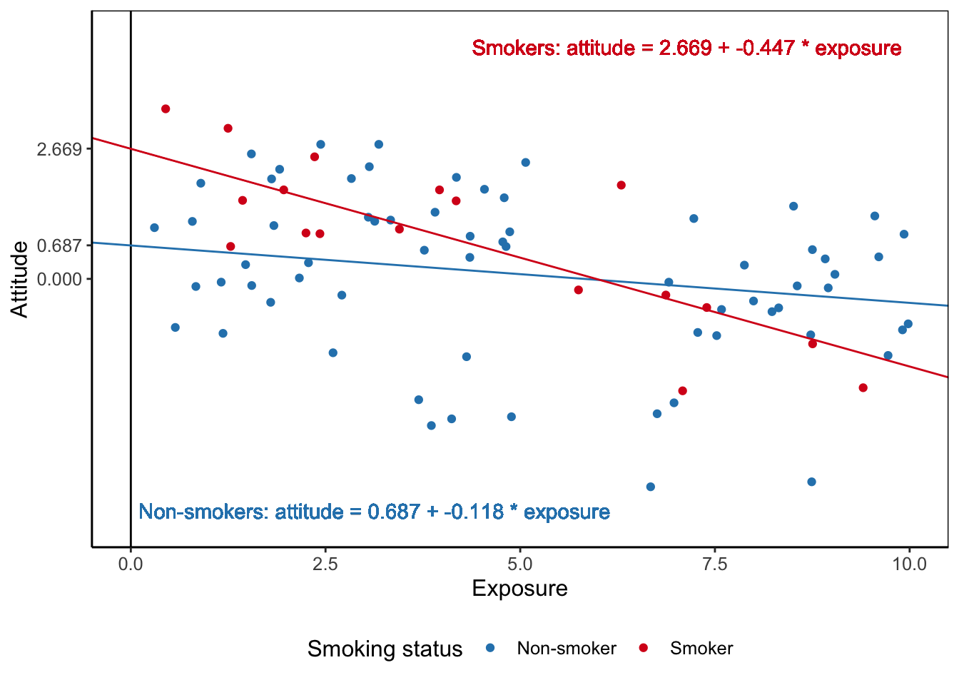
Figure 6.22: The effects of exposure on attitude for non-smokers and smokers. Both smokers and non-smokers are assumed to have average contact with smokers.