5.1 Different Means for Three or More Groups

Celebrity endorsement theory states that celebrities who publicly state that they favour a product, candidate, or cause, help to persuade consumers to adopt or support the product, candidate, or cause (for a review, see Erdogan, 1999; for an alternative approach, see McCracken, 1989).

Imagine that we want to test if the celebrity who endorses a fund raiser in a fund-raising campaign makes a difference to people’s willingness to donate. We will be using the celebrities George Clooney and Angelina Jolie, and we will compare campaigns with one of them to a campaign without celebrity endorsement.

Figure 5.1: George Clooney and Angelina Jolie. Photo Clooney by Angela George CC BY-SA 3.0. Photo Jolie by Foreign and Commonwealth Office CC BY 2.0, via Wikimedia Commons.

Let us design an experiment to investigate the effects of celebrity endorsement. We sample a number of people (participants), whom we assign randomly to one of three groups. We show a campaign video with George Clooney to one group, a video with Angelina Jolie to another group, and the third group (the control group) sees a campaign video without celebrity endorsement. So we have three experimental conditions (Clooney, Jolie, no endorser) as our independent variable.

Our dependent variable is a numeric scale assessing the participant’s willingness to donate to the fund raiser on a scale from 1 (“absolutely certain that I will not donate”) to 10 (“absolutely certain that I will donate”). We will compare the average outcome scores among groups. If groups with Clooney or Jolie as endorser have systematically higher average willingness to donate than the group without celebrity endorsement, we conclude that celebrity endorsement has a positive effect.

In statistical terminology, we have a categorical independent (or predictor) variable and a numerical dependent variable. In experiments, we usually have a very limited set of treatment levels, so our independent variable is categorical. For nuanced results, we usually want to have a numeric dependent variable. Analysis of variance was developed for this kind of data (R. A. Fisher, 1919), so it is widely used in the context of experiments.

5.1.1 Mean differences as effects

Figure 5.2 shows the willingness to donate scores for twelve participants in our experiment. Four participants saw Clooney, four saw Jolie, and four did not see a celebrity endorser in the video that they watched.

Figure 5.2: How do group means relate to effect size?

A group’s average score on the dependent variable represents the group’s score level. The group averages in Figure 5.2 tell us for which celebrity the average willingness to donate is higher and for which situation it is lower.

Random assignment of test participants to experimental groups (e.g., which video is shown) creates groups that are in principle equal on all imaginable characteristics except the experimental treatment(s) administered by the researcher. Participants who see Clooney should have more or less the same average age, knowledge, and so on as participants who see Jolie or no celebrity. After all, each experimental group is just a random sample of participants.

If random assignment was done successfully, differences between group means can only be caused by the experimental treatment (we will discuss this in more detail in Chapter 8). Mean differences are said to represent the effect of experimental treatment in analysis of variance.

Analysis of variance was developed for the analysis of randomized experiments, where effects can be interpreted as causal effects. Note, however, that analysis of variance can also be applied to non-experimental data. Although mean differences are still called effects in the latter type of analysis, these do not have to be causal effects.

In analysis of variance, then, we are simply interested in differences between group means. The conclusion for a sample is easy: Which groups have higher average score on the dependent variable and for which are they lower? A means plot, such as Figure 5.3, aids interpretation and helps communicating results to the reader. On average, participants who saw Clooney or Jolie have higher willingness to donate than participants who did not see a celebrity endorser.

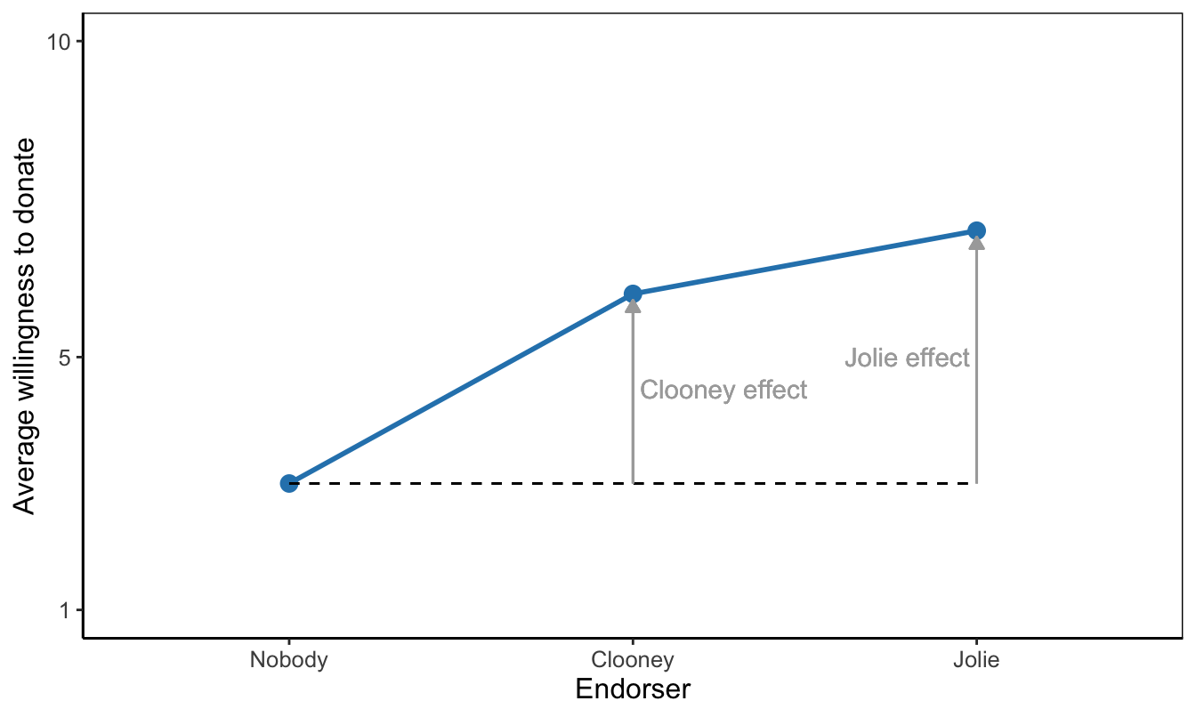
Figure 5.3: A means plot showing that average willingness to donate is higher with a celebrity endorser than without a celebrity endorser. As a reading instruction, effects of endorsers are represented by arrows.

Effect size in an analysis of variance refers to the overall differences between group means. We use eta² as effect size, which gives the proportion of variance in the dependent variable (willingness to donate) explained or predicted by the group variable (experimental condition).

This proportion is informative and precise. If you want to classify the effect size in more general terms, you should take the square root of eta² to obtain eta. As a measure of association, eta can be interpreted with the following rules of thumb:

• 0.1 (0 ≤ eta² < .2) = small or weak effect,
• 0.3 (.2 ≤ eta² < .4) = medium-sized or moderate effect,
• 0.5 (.4 ≤ eta²) = large or strong effect.

5.1.2 Between-groups variance and within-groups variance

For a better understanding of eta² and the statistical test of an analysis of variance model, we have to compare the individual scores to the group averages and to the overall average. Figure 5.4 adds overall average willingness to donate to the plot (horizontal black line) with participants’ scores and average experimental group scores (coloured horizontal lines).

Figure 5.4: Which part of score differences tells us about the differences between groups?

Let us assume that we have measured willingness to donate for a sample of 12 participants in our study as depicted in Figure 5.4. Once we have our data, we first have a look at the percentage of variance that is explained, eta². What does it mean if we say that a percentage of the variance is explained when we interpret eta²?

The variance that we want to explain consists of the differences between the scores of the participants on the dependent variable and the overall or grand mean of all outcome scores. Remember that a variance measures deviations from the mean. The dotted black arrows in Figure 5.4 express the distances between outcome scores and the grand average. Squaring, summing, and averaging these distances over all observations gives us the total variance in outcome scores.

The goal of our experiment is to explain why some of our participants have a willingness to donate that is far above the grand mean (horizontal black line in Figure 5.4) while others score a lot lower. We hypothesized that participants are influenced by the endorser they have seen. If an endorser has a positive effect, the average willingness should be higher for participants confronted with this endorser.

If we know the group to which a participant belongs—which celebrity she saw endorsing the fundraising campaign—we can use the average outcome score for the group as the predicted outcome for each group member—her willingness to donate due to the endorser she saw. The predicted group scores are represented by the coloured horizontal lines for group means in Figure 5.4.

Now what part of the variance in outcome scores (dotted black arrows in Figure 5.4) is explained by the experimental treatment? If we use the experimental treatment as predictor of willingness to donate, we predict that a participant’s willingness equals her group average (horizontal coloured line) instead of the overall average (horizontal black line), which we use if we do not take into account the participant’s experimental treatment.

So the difference between the overall average and the group average is what we predict and explain by the experimental treatment. This difference is represented by the solid black arrows in Figure 5.4. The variance of the predicted scores is obtained if we average the squared sizes of the solid black arrows for all participants. This variance is called the between-groups variance.

Playing with the group means in Figure 5.4, you may have noticed that eta² is high if there are large differences between group means. In this situation we have high between-groups variance—large black arrows—so we can predict a lot of the variation in outcome scores between participants.

In contrast, small differences between group averages allow us to predict only a small part of the variation in outcome scores. If all group means are equal, we can predict none of the variation in outcome scores because the between-groups variance is zero. As we will see in Section 5.1.3, zero between-groups variance is central to the null hypothesis in analysis of variance.

The experimental treatment predicts that a participant’s willingness equals the average willingness of the participant’s group. It cannot predict or explain that a participant’s willingness score is slightly different from her group mean (the red double-sided arrows in Figure 5.4). Within-groups variance in outcome scores is what we cannot predict with our experimental treatment; it is prediction error. In some SPSS output, it is therefore labeled as “Error”.

5.1.3 F test on the model

Average group scores tell us whether the experimental treatment has effects within the sample (Section 5.1.1). If the group who saw Angelina Jolie as endorser has higher average willingness to donate than the group who did not see an endorser, we conclude that Angelina Jolie makes a difference in the sample. But how about the population?

If we want to test whether the difference that we find in the sample also applies to the population, we use the null hypothesis that all average outcome scores are equal in the population from which the samples were drawn. In our example, the null hypothesis states that people in the population who would see George Clooney as endorser are on average just as willing to donate as people who would see Angelina Jolie or who would not see a celebrity endorser at all.

We use the variance in group means as the number that expresses the differences between group means. If all groups have the same average outcome score, the between-groups variance is zero. The larger the differences, the larger the between-groups variance (see Section 5.1.2).

We cannot just use the between-groups variance as the test statistic because we have to take into account chance differences between sample means. Even if we draw different samples from the same population, the sample means will be different because we draw samples at random. These sample mean differences are due to chance, they do not reflect true differences between groups in the population.

We have to correct for chance differences and this is done by taking the ratio of between-groups variance over within-groups variance. This ratio gives us the relative size of observed differences between group means over group mean differences that we expect by chance.

Our test statistic, then, is the ratio of two variances: between-groups variance and within-groups variance. The F distribution approximates the sampling distribution of the ratio of two variances, so we can use this probability distribution to test the significance of the group mean differences we observe in our sample.

Long story short: We test the null hypothesis that all groups have the same population means in an analysis of variance. But behind the scenes, we actually test between-groups variance against within-groups variance. That is why it is called analysis of variance.

5.1.4 Assumptions for the F test in analysis of variance

There are two important assumptions that we must make if we use the F distribution in analysis of variance: (1) independent samples and (2) homogeneous population variances.

5.1.4.1 Independent samples

The first assumption is that the groups can be regarded as independent samples. As in an independent-samples t test, it must be possible in principle to draw a separate sample for each group in the analysis. Because this is a matter of principle instead of how we actually draw the sample, we have to argue that the assumption is reasonable. We cannot check the assumption against the data.

Here is an example of an argument that we can make. In an experiment, we usually draw one sample of participants and, as a next step, we assign participants randomly to one of the experimental conditions. We could have easily drawn a separate sample for each experimental group. For example, we first draw a participant for the first condition: seeing George Clooney endorsing the fundraising campaign. Next, we draw a participant for the second condition, e.g., Angelina Jolie. The two draws are independent: whomever we have drawn for the Clooney condition is irrelevant to whom we draw for the Jolie condition. Therefore, draws are independent and the samples can be regarded as independent.

Situations where samples cannot be regarded as independent are the same as in the case of dependent/paired-samples t tests (see Section 2.3.6). For example, samples of first and second observations in a repeated measurement design should not be regarded as independent samples. Some analysis of variance models can handle repeated measurements but we do not discuss them here.

5.1.4.2 Homogeneous population variances

The F test on the null hypothesis of no effect (the nil) in analysis of variance assumes that the groups are drawn from the same population. This implies that they have the same average score on the dependent variable in the population as well as the same variance of outcome scores. The null hypothesis tests the equality of population means but we must assume that the groups have equal dependent variable variances in the population.

We can use a statistical test to decide whether or not the population variances are equal (homogeneous). This is Levene’s F test, which is also used in combination with independent samples t tests. The test’s null hypothesis is that the population variances of the groups are equal. If we do not reject the null hypothesis, we decide that the assumption of equal population variances is plausible.

The assumption of equal population variances is less important if group samples are more or less of equal size (a balanced design, see Section 5.3.2). We use a rule of thumb that groups are of equal size if the size of the largest group is less than 10% (of the largest group) larger than the size of the smallest group. If this is the case, we do not care about the assumption of homogeneous population variances.

5.1.5 Which groups have different average scores?

Analysis of variance tests the null hypothesis of equal population means but it does not yield confidence intervals for group means. It does not always tell us which groups score significantly higher or lower.

Figure 5.5: Which groups have different average outcome scores in the population? The p values belong to independent-samples t tests on the means of two groups.

If the F test is statistically significant, we reject the null hypothesis that all groups have the same population mean on the dependent variable. In our current example, we reject the null hypothesis that average willingness to donate is equal for people who saw George Clooney, Angelina Jolie, or no endorser for the fund raiser. In other words, we reject the null hypothesis that the endorser does not matter to willingness to donate.

5.1.5.1 Pairwise comparisons as post-hoc tests

With a statistically significant F test for the analysis of variance model, several questions remain to be answered. Does an endorser increase or decrease the willingness to donate? Are both endorsers equally effective? The F test does not provide answers to these questions. We have to compare groups one by one to see which condition (endorser) is associated with a higher level of willingness to donate.

In a pairwise comparison, we have two groups, for instance, participants confronted with George Clooney and participants who did not see a celebrity endorse the fund raiser. We want to compare the two groups on a numeric dependent variable, namely their willingness to donate. An independent-samples t test is appropriate here.

With three groups, we can make three pairs: Clooney versus Jolie, Clooney versus nobody, and Jolie versus nobody. We have to execute three t tests on the same data. We already know that there are most likely differences in average scores, so the t tests are executed after the fact, in Latin post hoc. Hence the name post-hoc tests.

Applying more than one test to the same data increases the probability of finding at least one statistically significant difference even if there are no differences at all in the population. Section 4.7.3 discussed this phenomenon as capitalization on chance and it offered a way to correct for this problem, namely Bonferroni correction. We ought to apply this correction to the independent-samples t tests that we execute if the analysis of variance F test is statistically significant.

The Bonferroni correction divides the significance level by the number of tests that we do. In our example, we do three t tests on pairs of groups, so we divide the significance level of five per cent by three. The resulting significance level for each t test is .0167. If a t test’s p value is below .0167, we reject the null hypothesis, but we do not reject it otherwise.

5.1.5.2 Two steps in analysis of variance

Analysis of variance, then, consists of two steps. In the first step, we test the general null hypothesis that all groups have equal average scores on the dependent variable in the population. If we cannot reject this null hypothesis, we have too little evidence to conclude that there are differences between the groups. Our analysis of variance stops here, although it is recommended to report the confidence intervals of the group means to inform the reader. Perhaps our sample was just too small to reject the null hypothesis.

If the F test is statistically significant, we proceed to the second step. Here, we apply independent-samples t tests with Bonferroni correction to each pair of groups to see which groups have significantly different means. In our example, we would compare the Clooney and Jolie groups to the group without celebrity endorser to see if celebrity endorsement increases willingness to donate to the fund raiser, and, if so, how much. In addition, we would compare the Clooney and Jolie groups to see if one celebrity is more effective than the other.

5.1.5.3 Contradictory results

It may happen that the F test on the model is statistically significant but none of the post-hoc tests is statistically significant. This mainly happens when the p value of the F test is near .05. Perhaps the correction for capitalization on chance is too strong; this is known to be the case with the Bonferroni correction. Alternatively, the sample can be too small for the post-hoc test. Note that we have fewer observations in a post-hoc test than in the F test because we only look at two of the groups.

This situation illustrates the limitations of null hypothesis significance tests (Chapter 4.7). Remember that the 5 per cent significance level remains an arbitrary boundary and statistical significance depends a lot on sample size. So do not panic if the F and t tests have contradictory results.

A statistically significant F test tells us that we may be quite confident that at least two group means are different in the population. If none of the post-hoc t tests is statistically significant, we should note that it is difficult to pinpoint the differences. Nevertheless, we should report the sample means of the groups (and their standard deviations) as well as the confidence intervals of their differences as reported in the post-hoc test. The two groups that have most different sample means are most likely to have different population means.