4.2 Null Hypothesis Significance Testing

Null Hypothesis Significance Testing (NHST) is the most widely used method for statistical inference in the social sciences and beyond. The logic underlying NHST is called the Neyman Pearson approach (Lehmann, 1993). Though these names are not widely known, the work of Jerzy Neyman (1894–1981) and Egon Pearson (1895–1980) still has a profound impact on the way current research is conducted, reviews are considered, and papers are published.

The Neyman Pearson approach ensures tight control on the probability of making correct and incorrect decisions. It is a decision framework that gives you a clear criterion and also an indication of what the probability is that your decision is wrong. The decision in this regard, is either the acceptance or rejection of the \(H_0\) hypothesis.

The Neyman Pearson approach is about choosing your desired probability of making correct and incorrect decisions, setting up the right conditions for this, and making a decision. It considers the following:

Alpha - Determine your desired risk of drawing the wrong conclusion.
Power - Determine your desired probability of drawing the correct conclusion.
The true effect size
The sample size needed to achieve desired power.
Conduct your research with this sample size.
Determine the test statistic.
Determine if \(p\)-value \(\leq \alpha\). If so, reject \(H_0\).

The two decisions can be visualized in a \(2 \times 2\) table where in reality \(H_0\) can be true or false (\(H_A\) is true), and the decision can either be to reject \(H_0\) or not. Figure 4.3 illustrates the correct and incorrect decisions that can be made. The green squares obviously indicate that it is a good decision to reject \(H_0\) when it is in fact false, and not to reject \(H_0\) if it is in reality true. And the red squares indicate that it is a wrong decision to reject \(H_0\) when it is actually true (Type I error), or not reject \(H_0\) if it is in reality false (Type II error).

Figure 4.3: NHST decision table.

Intuitively it is easy to understand that you would want the probability of an incorrect decision to be low, and the probability of a correct decision to be high. But how do we actually set these probabilities? Let’s consider the amount of yellow candies from the candy factory again. In Chapter 1.2 we learned that the factory produces candy bags where one fifth of the candies are supposed to be yellow. Now suppose we don’t know this and our null hypothesis would be that half of the candies would be yellow. In Figure 1.4 you can set the parameter values to .5 and .2 and see what the discrete probability distributions look like.

As the candy factory produces bags with ten candies, we can look at both probability distributions. Figure 4.4 shows both distributions.

\(H_0\) Distribution
- Half of the candies in the bag are yellow
- The parameter of the candy machine is .5
- With expected value 5 out of 10

\(H_A\) Distribution
- One fifth of the candies in the bag are yellow
- The parameter of the candy machine is .2
- With expected value 2 out of 10

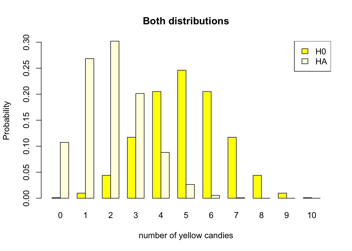
Figure 4.4: Discrete binomial distributions

We will use both distributions in Figure 4.4 to clarify the different components within the Neyman Pearson approach later in this chapter. For now, take a good look at both probability distributions, and consider a bag of candy containing 4 yellow candies. Are you able to determine if this bag is the result of a manufacturing process that produces bags with 20% or 50% yellow candies?

Doing research is essentially the same. You collect one sample, and have to determine if the effect of your study is non existent (\(H_0 = \text{true}\)) or that there is something going on (\(H_0 \neq \text{true}\)).

4.2.1 Alpha

The first step in the Neyman Pearson approach is to set the desired type I error rate, also known as the significance level, \(\alpha\). This is the probability of rejecting the null hypothesis when it is in reality true. In the \(2 \times 2\) decision table in Figure 4.5, this corresponds to the top left quadrant.

As a researcher, you decide how much risk you are willing to take to make a type I error. As the Neyman Pearson approach is a decision framework, you have to set this probability before you start collecting data. The most common value for \(\alpha\) is .05, which means that you accept a 5% chance of making a type I error of rejecting the null hypothesis when it is in reality true.

Figure 4.5: NHST decision table.

In our yellow candy example, assuming the null hypothesis to be true, relates to the parameter value of .5 and the associated probability distribution shown in Figure 4.1. We have already determined that if \(H_0\) is true, it is still possible we could get a bag with 0 or 10 yellow candies. Deciding to reject the null hypothesis in any of these cases, would be wrong, because the null hypothesis is assumed to be true. The exact probabilities can be found on the y-axis of Figure 4.1, and are also shown in the Table 4.1 below. Looking at the probability of getting 0 or 10 candies in Table 4.1, we see that together this amounts to .002 or 0.2%. If we would decide to only reject the null hypothesis if we would get 0 or 10 candies, this would be a wrong decision, but we would also know that the chance of such a decision is pretty low. Our type I error, alpha, significance level, would be .002.

Table 4.1: Probabilities of drawing a certain amount of yellow candies from a bag of 10 candies, assuming the null hypothesis to be true.
#Y	0	1	2	3	4	5	6	7	8	9	10
Pr H0	0.001	0.010	0.044	0.117	0.205	0.246	0.205	0.117	0.044	0.010	0.001

Choosing such an alpha level would result in a threshold between 0 and 2 and 9 and 10. We call this the critical value associated with the chosen alpha level. Where on the outside of the threshold we would reject the null hypothesis, and inside the threshold we would not reject the null hypothesis. So, if that is our decision criterion, we would reject the null hypothesis if we would draw a bag with 0 or 10 yellow candies, and not reject the null hypothesis if we would draw a bag with 1, 2, 3, 4, 5, 6, 7, 8, or 9 yellow candies. Amounting to a type I error rate of .002 or 0.2%. Figure 4.6 shows the critical values for the null hypothesis distribution, and indicate what the decision would be for values on the outside and inside of the decision boundary.

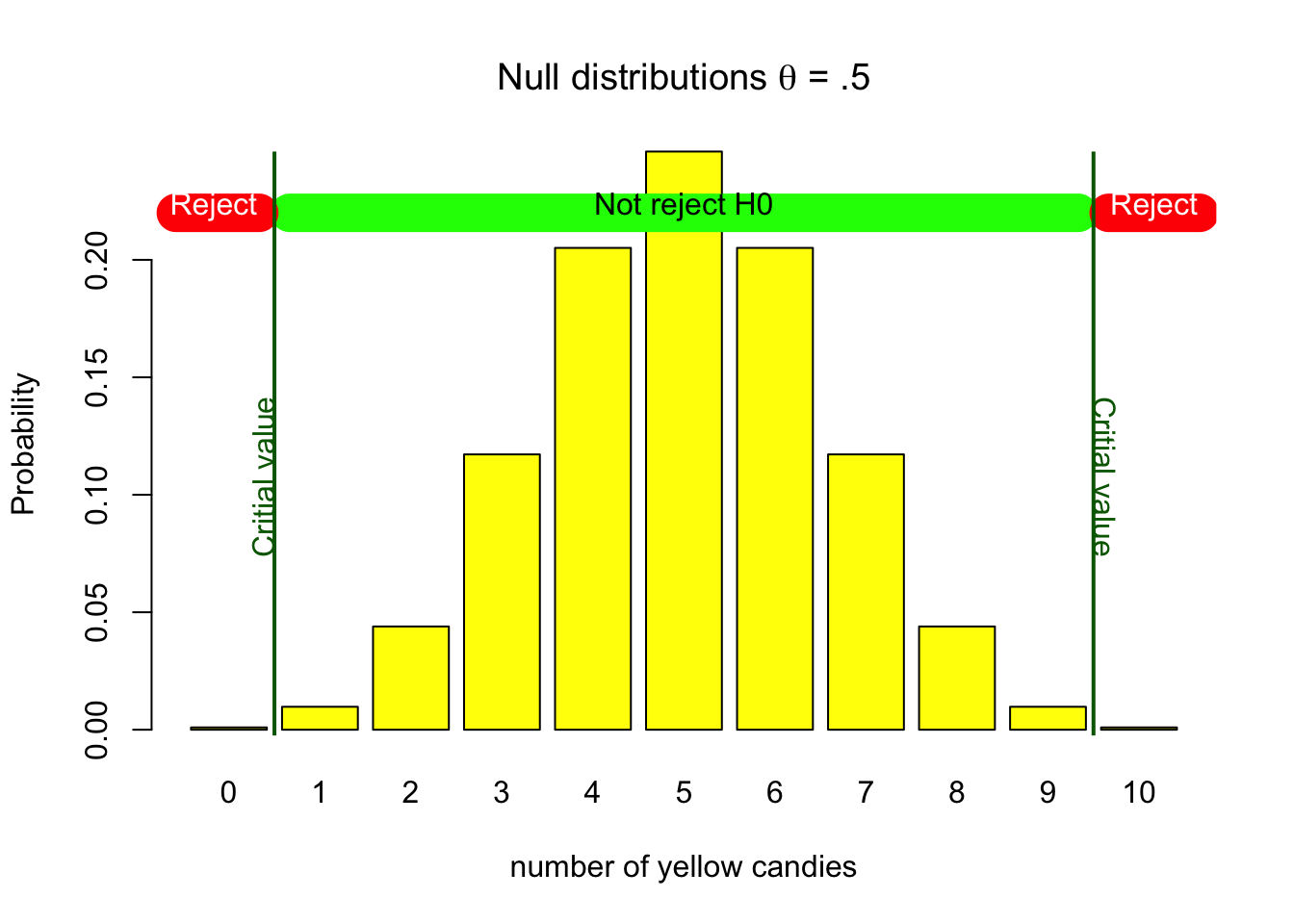
Figure 4.6: H0 binomial distribution with critical values

In the social sciences, we allow ourselves to make a wrong decision more often. We usually set the alpha level to .05. For our discrete example setting the alpha level to .05 is not really possible. Looking at Table 4.1, we could raise the significance level to .044 if we would reject the null hypothesis if we would draw 0, 1, 2 or 8, 9, 10 yellow candies. This would result in a type I error rate of 4.4%. Though if we would also reject the null hypothesis with 3 or 7 yellow candies, we would have a type I error rate of 5.7%. For a discrete probability distribution with a limited number of outcomes, it is not always possible to set the alpha level exactly to .05.

For continuous probability distributions, such as the normal distribution, it is possible to set the alpha level to exactly .05. For example the null hypothesis that average media literacy in the population of children equals 5.5 on a scale from one to ten.

For such continuous variables, we can estimate a sampling distribution around the hypothesized population value using a theoretical approach (Chapter 2.3). Remember (Section 1.2.4) that the population value is the expected value of the sampling distribution, that is, its mean (if the estimator is unbiased). The sampling distribution, then, is centered around the population value specified in the null hypothesis. This sampling distribution tells us the probabilities of all possible sample outcomes if the null hypothesis is true. It allows us to identify the most unlikely samples. In Step 2 in Figure 4.7, we set the alpha level to .05. This means that we cut off 2.5% of the area in each tail of the sampling distribution. The critical values are the values that separate the 2.5% of the area in each tail from the 95% of the area in the middle. If we assume the population parameter to be 5.5, rejecting the null hypothesis would again be a wrong decision. Thus setting the boundary by using an alpha level of .05, would yield a wrong decision in 5% of the samples we take. Just like the discrete candy color case, we decide to reject \(H_0\) on the outside of the critical value and not reject \(H_0\) on the inside of the critical value. In Step 4 in Figure 4.7, we add the result of a sample. You can redraw multiple samples by clicking the button in the app.

Note that the reasoning for the discrete case and the continuous case is the same. The only difference is that for the continuous case we can set the alpha level exactly to .05.

Figure 4.7: Sampling distribution of average media literacy according to the null hypothesis.

4.2.2 1 - Alpha

The decision to not reject the null hypothesis when it is in reality true is indicated by \(1 - \alpha\). It does not go by any other name, but in terms of probability, it is directly dependent on your desired type I error rate, your chosen alpha level. It therefore corresponds to the probabilities in Table 4.1 of 1, 2, 3, 4, 5, 6, 7, 8, or 9 yellow candies in the candy factory example. We have a 99.8% (1 - .002) chance of making the correct decision to not reject \(H_0\) when we assume it to be true. The inside of the critical value in Figure 4.6 is the area where we do not reject the null hypothesis. In the \(2 \times 2\) decision table in Figure 4.3, this corresponds to the bottom left green quadrant.

Now that we have determined our critical value (for our particular sample size) based on our desired alpha, significance level, we can use this critical value to look at the power.

4.2.3 Power

The power is the probability of making the correct decision to reject the null hypothesis when it is in fact false. In the \(2 \times 2\) decision table in Figure 4.3, this corresponds to the top right quadrant. As we have already set our decision criterion by choosing our alpha level in the previous step, we already know when we decide to reject the null hypothesis. In figure (fig:nulldistributionalpha) we determined our type I error could be 0.2%, if we would reject the null hypothesis if we would draw 0 or 10 yellow candies. The critical value would in that case be between 0 and 1 and 9 and 10. We use this same critical value to determine the power of the test, as it establishes our decision boundary.

As the right column of Figure 4.3 only states that \(H_0 = \text{FALSE}\), it does not state what this entails. Within the Neyman Pearson approach, this would be the true population value with its associated probability distribution. We already established that this would be the distribution with a parameter value of .2. In Figure 4.8, we see that our decision criterion is still the same. That we decide to reject the null when we sample 0 or 10 yellow candies. But the distribution has now changed.

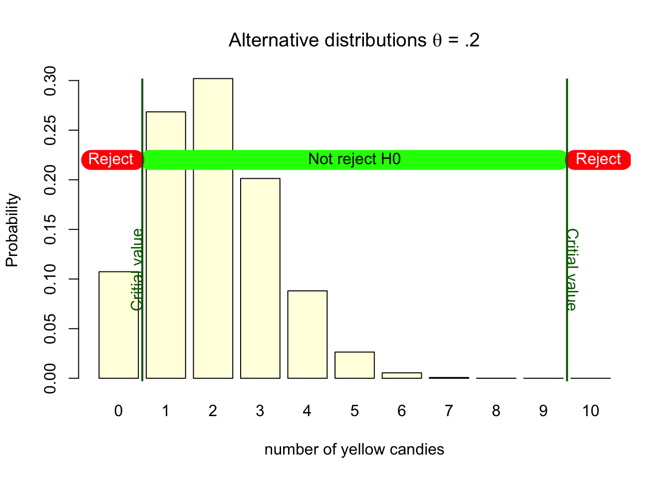
Figure 4.8: HA binomial distributions with critical values

If this alternative distribution would actually be true, deciding to reject the null would be a good decision. Though, we can also see that if this alternative is true, if the parameter truly is .2, getting a bag with 0 or 10 yellow candies does not happen that often. The probabilities for 10 yellow candies is almost none, and the probability for getting 0 yellow candies is about 11%. This means that if the alternative hypothesis is true, if our sample originates from the alternative hypothesis, we would only make the decision to reject the null hypothesis in 11% of the samples we get out of it. So, the power of the test, correctly rejecting the null when this specific alternative is true is only 11%.

The only way to increase the power is to increase the sample size of the study, or increase the type I error.

As stated earlier we would rather have a higher probability of making the correct decision. In the social sciences we are striving for a power of .80. This means that we want to make the correct decision in 80% of the cases when the null hypothesis is false. In our candy factory example, this would mean that we would want to reject the null hypothesis in 80% of the replications. With our machine producing bags with 10 candies, this is just not possible. The only way to increase the power is to increase the sample size of the study. In the candy factory example, this would mean that we would have to increase the number of candies in the candy bags. We will come back to this in the Chapter 4.2.11 on sample size.

One more thing to note, is that the true power of the test can only be determined if you know the true population value. In practice, we do not know if the null or the alternative hypothesis is true. We can only calculate the power of the test when we assume some alternative hypothesis. It is good practice to base your assumptions about the alternative hypothesis on previous research, theory, or other empirical evidence. This is mostly expressed as the expected effect size, the expected difference between the null and the alternative hypothesis.

In all statistical software, the power of the test is not calculated based on the true effect size, but on the found effect size in your sample. This is called the observed power and will be covered in Chapter 4.2.8.

4.2.4 Beta

The probability of making a type II error is indicated by \(\beta\). It is the probability of not rejecting the null hypothesis when it is in reality false. In the \(2 \times 2\) decision table in Figure 4.3, this corresponds to the bottom right quadrant. The power of the test is \(1 - \beta\). In our candy factory example, the power of the test is .11, so the probability of making a type II error is .89. It is the sum of the probabilities of getting 1, 2, 3, 4, 5, 6, 7, 8, or 9 yellow candies, when the machine actually produces bags with 2 yellow candies with the corresponding probabilities as shown in Figure 4.8.

4.2.5 Test statistic

In Chapter 1.2.1 we discussed the sample statistic, and defined it as any value describing a characteristic of the sample. This could be the mean, or the proportion, or the correlation, or the regression coefficient. It is a value that is calculated from the sample. Note that conversions of the sample statistic, such as the difference between two sample means, or the ratio of two sample variances, \(t\)-values, \(F\)-values, and \(\chi^2\)-values are also sample statistics.

The test statistic is a sample statistic that is used to test the null hypothesis. In our candy factory example, the test statistic would be the number of yellow candies in the bag we sample. If we would draw a bag with 4 yellow candies, the test statistic would be 4.

In the previous sections, we have determined our decision criterion, the critical value, based on our desired alpha level. We have also determined the power of the test, based on the alternative hypothesis. The test statistic is used to determine if we reject the null hypothesis or not. If the test statistic is equal to the critical value or more extreme, we reject the null hypothesis. If the test statistic is inside the critical value, we do not reject the null hypothesis.

Looking at Figure 4.6, we see that the critical value is between 0 and 1 and 9 and 10. If we would draw a bag with 4 yellow candies, we can check if the value 4 is inside or outside the critical value. As 4 is inside the critical value, we would not reject the null hypothesis.

The test statistic is the value that is used to decide if we reject the null hypothesis or not.

For continuous variables, as described in Figure 4.7, the test statistic is the sample mean. If the sample mean is outside the critical value, we reject the null hypothesis. If the sample mean is inside the critical value, we do not reject the null hypothesis. If you select Step 4 in Figure 4.7, and draw a few samples, you can see if the test statistic, the sample mean, is inside or outside the critical value. Again, the reasoning for continuous variables is the same as for the discrete variables.

4.2.6 P-value

We have learned that a test is statistically significant if the test statistic is in the rejection region. Statistical software, however, usually does not report the rejection region for the sample statistic. Instead, it reports the p-value of the test, which is sometimes referred to as significance or Sig. in SPSS.

The p-value is the probability of obtaining a test statistic at least as extreme as the result actually observed, under the assumption that the null hypothesis is true.

In the previous section we considered a sample with 4 yellow candies. The p-value gives the probability of randomly drawing a sample that is as extreme or more extreme than our current sample assuming that the null hypothesis is true. “As extreme or more extreme” here means as far or further removed from the value specified by the null hypothesis. Concretely, in our case that means the probability of drawing a sample with 4 or fewer yellow candies. The p-value considers the probability of such a sample, but also ads the probability of getting a sample with less yellow candies. This is what is meant with “at least as extreme”. this is not really intuitive, but it refers to the less likely test statistics, iIn our case 0, 1, 2 and 3, are even less probable than 4 yellow candies. The assumption that the null hypothesis is true indicates that we need to look at the probabilities from the sampling distribution that is created based on the null distribution hypothesis. Looking at Table 4.1, we see that the probability of drawing a random sample with 0, 1, 2, 3 or 4 yellow candies under the null distribution is 0.001 + 0.010 + 0.044 + 0.117 + 0.205 = 0.377 according to the sampling distribution belonging to the null hypothesis. This 0.377 is the p-value. The conditional (conditional on H0 being true) probability of getting a sample that is as or less likely than the test statistic that we have of our current sample.

Rejecting the null hypothesis does not mean that this hypothesis is false or that the alternative hypothesis is true. Please, never forget this.

The reasoning applied when comparing our test statistic to the critical value is the same as when comparing the p-value to the alpha level. If the p-value is smaller or equal to than the alpha level, we reject the null hypothesis. If the p-value is larger than the alpha level, we do not reject the null hypothesis.

If the test statistic is within the critical values, the p-value is always larger than the alpha level. If the test statistic lies outside the critical value, the p-value is always smaller than the alpha level. In the case that the test statistic is exactly the same as the critical value, the p-value is exactly equal to the alpha level, we still decide to reject the null hypothesis.

Reject \(H_0\) when \(p\)-value \(\leq \alpha\)

As both the p-value and the alpha level assume the null to be true, you can find both probabilities under the null distribution. For continuous variables, the p-value is the area under the curve of the probability distribution that is more extreme than the sample mean. The significance level is chosen by you as a researcher and is fixed.

It is important to remember that a p-value is a probability under the assumption that the null hypothesis is true. Therefore, it is a conditional probability.

Compare it to the probability that we throw sixes with a dice. This probability is one out of six under the assumption that the dice is fair. Probabilities rest on assumptions. If the assumptions are violated, we cannot calculate probabilities.

If the dice is not fair, we don’t know the probability of throwing sixes. In the same way, we have no clue whatsoever of the probability of drawing a sample like the one we have if the null hypothesis is not true in the population.

Figure 4.9 shows a t-distribution, which represents the null distribution. A statistical test was set up with an alpha level of 5% (red area). The and the p-value (blue area) indicates the probability of drawing a random sample with a t-value of 2 or values that are even further removed from the null hypothesis (more extreem). The figure shows what this test would look like for a two sided test (left) and a one two sided hypothesis test (right). We will cover one and two sided testing in Chapter 4.2.12. For now, just notice that, looking at the left graph, the p-value is greater than 0.05, because the test statistic is not as or more extreme than the critical value. In other words, the test is not significant. In the one-sided test depicted on the right, the p-value lies in the rejection region and is, thus, significant.

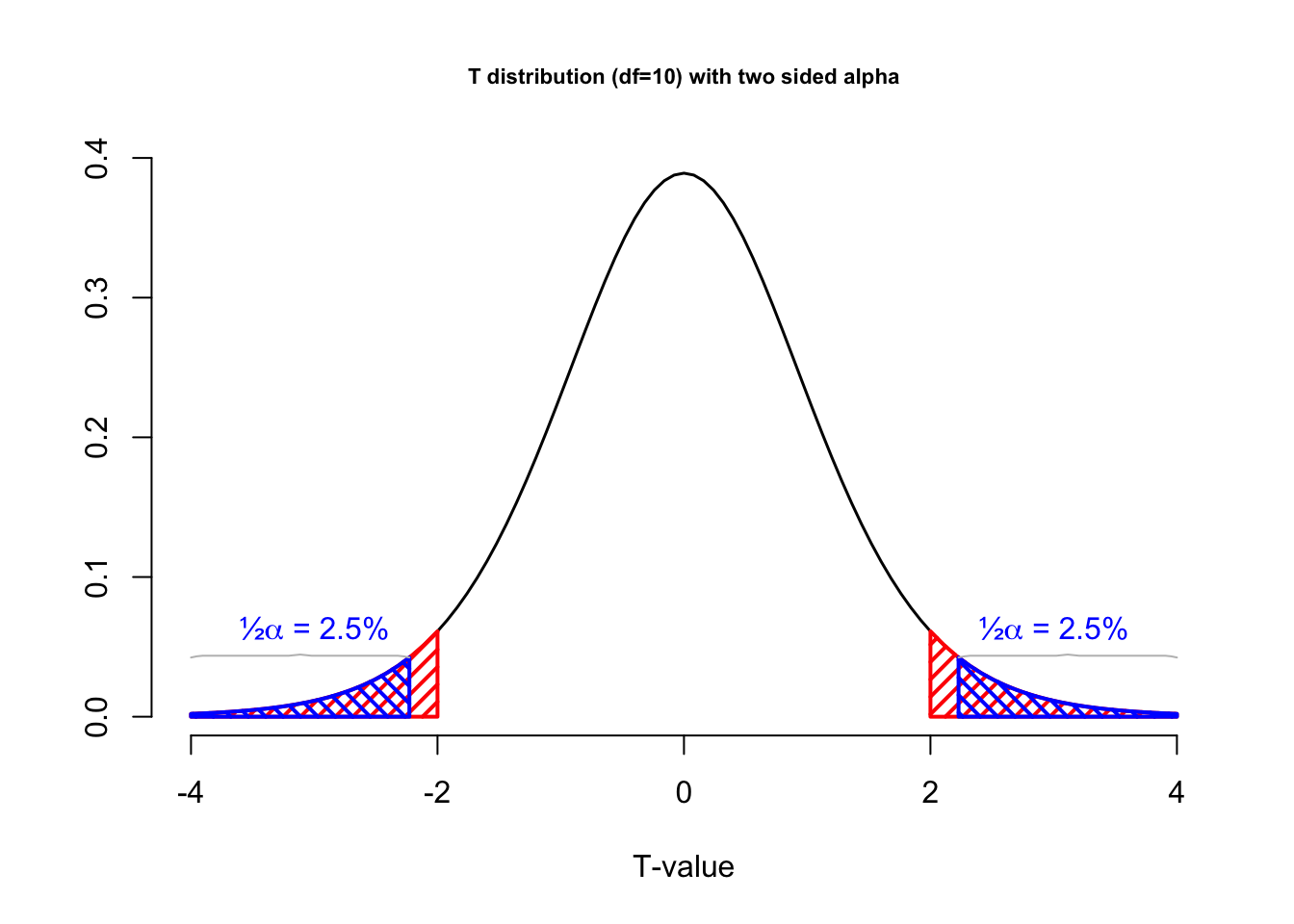
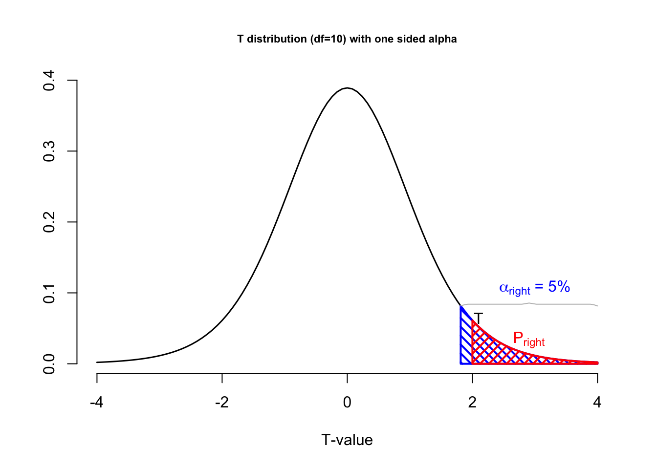
Figure 4.9: T-distributions with alpha level and p-value

In Figure 4.9, the blue vertical boundaries represent the critical value associated with a chosen alpha level of 5%, the blue area under the curve. The red vertical line represents the t-value from the sample, which in this example was 2. The red area under the curve represents the p-value, the probability of getting this t-value or more extreme.

Figure 4.10 represents the sampling distribution of average media literacy. You can take a sample and play around with the population mean according to some null hypothesis. If the mean in the sample is outside the critical value, it falls in the alpha rejection region.

Figure 4.10: Sampling distribution of average media literacy according to the null hypothesis.

The reasoning is again the same as for discrete variables. If the p-value is smaller or equal to the alpha level, we reject the null hypothesis. If the p-value is larger than the alpha level, we do not reject the null hypothesis.

4.2.7 True effect size

The true effect size is the difference between the null hypothesis and the true population value. This can also be expressed in terms of the test statistic. For example, if the IQ scores for communication science students are 120 in the population, the true affect size can be expressed as 20 IQ points, but also as a t-value. The true effect size denotes the genuine effect within the population, representing the actual difference, correlation, or parameter value.

In the candy factory example, the true effect size is .5 - .2 = .3. This is the difference in the proportion of yellow candies in the bags. In Figure 4.11 you can see the difference in the two distributions. The true effect size is the difference in the expected value of the two distributions. In absolute terms, it is 5 - 3 expected number of yellow candies in the bag. In terms of the parameter it is the proportion .5 - .2.

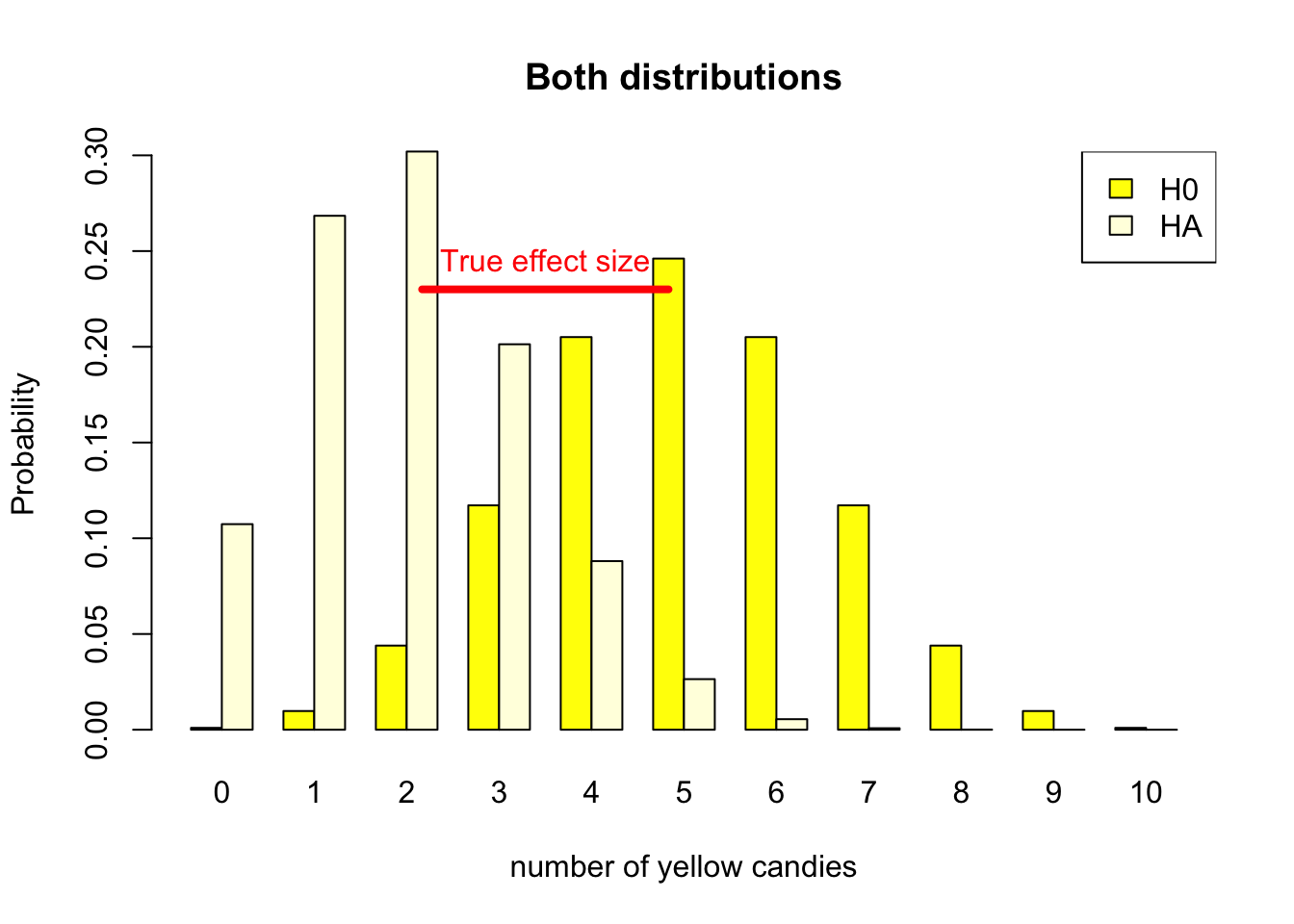
Figure 4.11: Discrete binomial distributions

True refers to the actual difference in the population, which is unknown to us. In our candy factory example, we can only observe the sample from a candy bag and make assumptions based on the null and alternative hypotheses.

Depending on the true value in the population, a true effect size could be small, medium, or large. In order to detect small true effect sizes, we need a large sample size. A larger sample offers more precision, so the difference between our sample outcome and the hypothesized value is more often sufficient to reject the null hypothesis. For example, we would reject the null hypothesis that average candy weight is 2.8 grams in the population if average weight in our sample bag is 2.70 grams and our sample is large. But we may not reject this null hypothesis if we have the same outcome in a small sample bag.

The larger our sample, the more sensitive our test will be, so we will get statistically significant results more often. If we think of our statistical test as a security metal detector, a more sensitive detector will go off more often.

4.2.7.1 Practical relevance

Investigating the effects of a new medicine on a person’s health, we may require some minimum level of health improvement to make the new medicine worthwhile medically or economically. If a particular level of improvement is clinically important, it is practically relevant (sometimes called practically significant).

If we have decided on a minimum level of improvement that is relevant to us, we want our test to be statistically significant if the average true health improvement in the population is at least of this size. We want to reject the null hypothesis of no improvement in this situation.

A larger sample size makes a statistical test more sensitive. The test will pick up (be statistically significant for) smaller effect sizes.
A larger effect size is more easily picked up by a statistical test. Larger effect sizes yield statistically significant results more easily, so they require smaller samples.

For media interventions such as health, political, or advertisement campaigns, one could think of a minimum change of attitude affected by the campaign in relation to campaign costs. A choice between different campaigns could be based on their efficiency in terms of attitudinal change per cost unit.

Note the important difference between practical relevance and statistical significance. Practical relevance is what we are interested in. If the new medicine is sufficiently effective, we want our statistical test to signal it. In the security metal detector example: If a person carries too much metal, we want the detector to pick it up.

Statistical significance is just a tool that we use to signal practically relevant effects. Statistical significance is not meaningful in itself. For example, we do not want to have a security detector responding to a minimal quantity of metal in a person’s dental filling. Statistical significance is important only if it signals practical relevance. We will return to this topic in Chapter 4.2.11 on sample size.

4.2.8 Observed effect size

In Chapter 4.2.7 we discussed the true effect, the difference between the null hypothesis and the true alternative hypothesis. The problem is that we do not know the true effect, we do not know which of the two hypothesis is actually true.

We can only estimate the true effect using the sample statistic. The difference between the sample statistic and the null hypothesis is called the observed effect size. In the candy factory example, the observed effect size is the difference between the number of yellow candies in the sample and the number of yellow candies in the null hypothesis. If the null hypothesis is that the machine produces bags with 5 yellow candies, and the sample contains 4 yellow candies, the observed effect size is 1.

The same definition holds for the continuous case. If the null hypothesis is that the average media literacy in the population is 5.5, and the sample mean is 3.9, the observed effect size is 1.6. Or if we hypothesize that average candy weight in the population is 2.8 grams and we find an average candy weight in our sample bag of 2.75 grams, the effect size is -0.05 grams. If a difference of 0.05 grams is a great deal to us, the effect is practically relevant.

Note that the effect sizes depend on the scale on which we measure the sample outcome. The unstandardized effect size of average candy weight changes if we measure candy weight in grams, micro grams, kilograms, or ounces. Of course, changing the scale does not affect the meaning of the effect size but the number that we are looking at is very different: 0.05 grams, 50 milligrams, 0.00005 kilos, or 0.00176 ounces. For this reason, we do not have rules of thumb for interpreting these unstandardized effect sizes in terms of small, medium, or large effects. But we do have rules of thumb for standardized effect sizes. Unstandardized effect sizes are very useful for reporting the practical results of your study, but they are not very useful for comparing studies or for meta-analysis.

You can imagine that estimating the true effect size on just one sample is not very reliable. The observed effect size could be the result of our sample being the result of the null being true, or the alternative being true. The way researchers try to get a notion of the true effect size is by replicating the study. If the observed effect size is consistent over multiple replications, we can be more confident that the average observed effect size is the true effect size. This is what we will cover in Chapter 4.2.10 about meta analysis.

4.2.8.1 Cohen’s d

In scientific research, we rarely have precise norms for raw differences (unstandardized effects) that are practically relevant or substantial. For example, what would be a practically relevant attitude change among people exposed to a health campaign?

To avoid answering this difficult question, we can take the variation in scores (standard deviation) into account. In the context of the candies example, we will not be impressed by a small difference between observed and expected (hypothesized) average candy weight if candy weights vary a lot. In contrast, if candy weight is quite constant, a small average difference can be important.

For this reason, standardized effect sizes for sample means divide the difference between the sample mean and the hypothesized population mean by the standard deviation in the sample. Thus, we take into account the variation in scores. This standardized observed effect size for tests on one or two means is known as Cohen’s d. Equation (4.3) illustrates how the sample mean \(\bar{x}\) is compared to the hypothesized population mean \(\mu_{H_0}\), and how this difference is standardized by deviding through the standard deviation \(s\). In appendix 9.9 we will cover the calculation of the paired and independent t-tests.

\[\begin{equation} d = \frac{\bar{x} - \mu_{H_0}}{s_x} \tag{4.3} \end{equation}\]

Using an inventory of published results of tests on one or two means, Cohen (1969) proposed rules of thumb for standardized effect sizes (ignore a negative sign if it occurs):

0.2: weak (small) effect,
0.5: moderate (medium) effect,
0.8: strong (large) effect.

Note that Cohen’s d can take values above one. These are not errors, they reflect very strong or huge effects (Sawilowsky, 2009).

4.2.8.2 Association as effect size

Measures of association such as Pearson’s product-moment correlation coefficient or Spearman’s rank correlation coefficient express effect size if the null hypothesis expects no correlation in the population. If zero correlation is expected, a correlation coefficient calculated for the sample expresses the difference between what is observed (sample correlation) and what is expected (zero correlation in the population).

Effect size is also zero according to the standard null hypotheses used for tests on the regression coefficient (b), R² for the regression model, and eta² for analysis of variance. As a result, we can use the standardized regression coefficient (Beta in SPSS and b* according to APA), R², and eta² as standardized effect sizes.

Because they are standardized, we can interpret their effect sizes using rules of thumb. The rule of thumb for interpreting a standardized regression coefficient (b*) or a correlation coefficient, for example, could be:

Very weak: between 0 and .10
Weak: between .10 and .30
Moderate: between .30 and .50
Strong: between .50 and .80
Very strong: between .80 and 1.00
Perfect association: 1.00

Note that we ignore the sign (plus or minus) of the effect when we interpret its size.

4.2.9 Post hoc power

Just as the observed effect size is based on the test statistic acquired from your sample, so is the post hoc power. It is also known as: observed, retrospective, achieved power (O’Keefe, 2007).

The power of a test assuming a population effect size equal to the observed effect size in the current sample.

— (O’Keefe, 2007)

The post hoc power refers to the probability of rejecting the null hypothesis assuming the alternative hypothesis has a population mean equal to the observed sample mean or more accurately the observed test statistic.

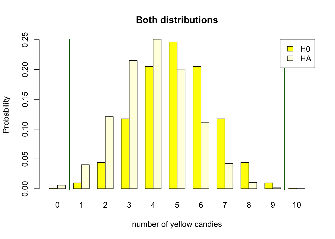
Figure 4.12: Discrete binomial distributions showing post hoc power

Figure 4.12 shows the post hoc power for a sample of 10 candies. The null hypothesis is that the machine produces bags with 5 yellow candies. The alternative hypothesis is that the machine produces bags with 2 yellow candies. But the post hoc power assumes the found test statistic of 4 candies to be the alternative population parameter of .4. Following the same decision criterion as defined in the previous sections, the post hoc power is almost zero. This is the probability of 0 or 10 yellow candies under the alternative distribution when rejecting the null hypothesis on the outside of the critical values.

You can imagine that if we look at a different candy bag and we would find 7 yellow candies, the post hoc power would not be the same. The post hoc power does not have much practical use, though SPSS produces this when you ask it, it is obvious that multiple replications of a research study will yield different results. As the true population mean is not a random variable, the actual power is fixed and should not vary.

4.2.10 Meta analysis

As mentioned in Chapter 4.2.8, the observed effect size is based on the sample statistic, and is likely to differ with every sample you take. If our research hypothesis is actually true, a random sample from a population described by the sampling distribution of the alternative hypothesis would be mot likely to result in us holding a bag with 2 yellow candies. But as we have seen in Figure 4.2, getting 4 yellow candies is reasonably probable as well.

Now imagine that we would take multiple samples, and calculate the observed effect size for each sample. If we would plot these observed effect sizes, we would get a distribution of observed effect sizes.

In research we can conduct replication studies to see if the observed effect size is consistent over multiple replications. If this is the case, we can be more confident that the average observed effect size is the true effect size and we can determine the true population mean. As we have seen in Chapter 1, it is in practical to draw many number of samples to create a sampling distribution. But we can use the results from multiple studies to get an indication of the true population mean.

Imagine that we get a hundred bags of candy (100 replications) and we consistently find 7 to 9 yellow candies, this would give us an indication of the true effect size being 8. It would also indicate that our initial alternative hypothesis is highly unlikely. This is essentially what meta analysis is about. Collecting effect sizes from multiple studies and combining them to get an indication of the true effect size.

Meta-analysis is a good example of combining research efforts to increase our understanding. It is useful to obtain more precise estimates of population values or effects. Meta-analysis is strongly recommended as a research strategy by Geoff Cumming, who coined the concept New Statistics. See Cumming’s book (2012), website, or YouTube channel if you are curious to learn more.

4.2.11 Sample size

As stated in Chapter 4.2.3, the only way to increase the power of a test is to increase the sample size. In the candy factory example, the sample size is the total number of candies in the bag. With only 10 candies in the bag, the power of the test is only 0.11. To reach our desired power of 80%, we clearly need to increase the sample size. In Figure 4.13, we increased the number of candies in the bag to 20. We can see on the x-axis that the possible outcome space for the number of yellow candies in the bag is now 0 to 20. This still assumes our \(H_0\) to be true, and the parameter of the machine is still \(\theta = .5\), half of the candies in the bag should be yellow. Though the parameter is still the same, the expected value when we have bags of 20 candies is now \(.5 \times 20 = 10\), right in the middle of our distribution.

Figure 4.13 still follows the reasoning scheme we have setup earlier. We decide to reject \(H_0\) on the outside of our critical values (Red vertical line). We determined the position of the critical value based on our chosen alpha level. Because our outcome space is larger we can be more accurate in striving for an \(\alpha = .05\). Our alpha is now 4.1%, we get this by adding the yellow bars 0, 1, 2, 3, 4, 5 and 15 up until 20, under the null distribution. This is not exactly 5 percent, but shifting the critical value inwards, would make the alpha level to high. So, this is close enough.

With this sample size, we can acquire our desired power of 80%. If we would assume our alternative hypothesis to be true, our decision to reject the null when you get 5 or less yellow candies, would be correct 80% of the time. The power of 80% is the sum of the light yellow bars under the assumption that \(H_A\) is true on the outside of our critical value. So, the power is the probability of getting 0, 1, 2, 3 ,4 ,5 or 15, 16,17, 18, 19 ,20 yellow candies under the alternative distribution.

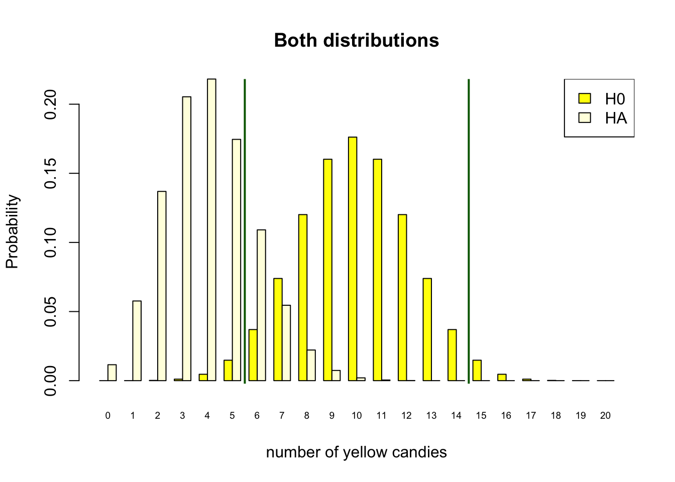
Figure 4.13: Discrete binomial distributions

The same reasoning is applied when using continuous sample statistics. Let’s revisit the candy weight example. We could have a null hypothesis that the average yellow candy weight is the same as the weight of all other candy colors. But if in reality the yellow candies would be heavier, let’s say with an effect size of .3, we would need to determine what sample size we would need to get a power of 80% and a alpha of 5%.

Figure 4.14 shows the relation between sample size, power, alpha and effect size. You can play around with the sliders de determine what sample size you would need to obtain a power of 80% for an effect size of .3.

Figure 4.14: How does test power depend on effect size, type of test, significance level, and sample size? Sampling distributions of the sample mean under the null hypothesis (H₀, left-hand curve) and under the assumed true value of the population mean (H₁, right-hand curve) for a one-sample t test.

For continuous sample statistics, we choose an alpha level, and we can see the critical value in the null distribution. The alpha level of 5% is the area under the curve of the null distribution on the outside of the critical values. The power is the area under the alternative distribution that is outside the critical values.

The reasoning is again the same as in the discrete case, when we use categorical sample statistics. We first determine our desired alpha and power, make sure our sample size is large enough to get the desired power, for our effect size of interest. Then, when we collect our data, we can calculate our test statistic and determine if we can reject the null hypothesis or not, being confident that we will be wrong in our conclusion in 5% of the cases, and that we will be right in 80% of the cases when the alternative hypothesis is actually true.

4.2.11.1 How to determine sample size

As stated in Chapter 4.2.3 about the power of a test, we already considered that we do not know the parameter for the alternative distribution and that we therefore also don’t know the true effect size. We stated that you can make an educated guess about the true effect size based on previous research, theory, or other empirical evidence.

In research you can take these assumptions into account by conducting a power analysis. A power analysis is a statistical method to determine the sample size you need to get a desired power for a given effect size.

It can be difficult to specify the effect size that we should expect or that is practically relevant. If there is little prior research comparable to our new project, we cannot reasonably specify an effect size and calculate sample size. Though, if there are meta analyses available for your research topic of interest or you have the effect sizes from a few previous studies, you can use programs such as G*Power to calculate the sample size you need to get a desired power for a given effect size. G*Power is a stand alone program that can be downloaded for free from the internet, and is specifically designed to calculate the required sample size for a wide range of statistical tests.

Download G*Power here

In G*Power you can specify the test you want to conduct, the effect size you expect, the alpha level you want to use, and the power you want to achieve. G*Power will then calculate the sample size you need to get the desired power for the given effect size.

For our candy color example, we can use G*Power to calculate the sample size we need to get a power of 80% for a given effect size of .3.

Figure 4.15: Power analysis in G*Power for a binomial distribution

In Figure 4.15 you can see that for the binomial test we have set the proportion p1 to .5 (\(H_0\)) and the proportion p2 (\(H_A\)) to .2, indirectly setting the effect size to .3. We have set the alpha level to 5% and the power to 80%. By hitting the calculate button, G*Power will calculate the sample size we need. In this case we need 20 candies in the bag to get a power of 80%. The plot shows exactly the same information as in Figure 4.13, though with lines instead of bars.

As mentioned in Chapter 4.2.7 about the true effect size, the sensitivity of a test is determined by the sample size. The larger the sample size, the more sensitive the test will be. This means that if we want to detect a small effect size, we need a large sample size. If we want to detect a large effect size, we can suffice with a smaller sample.

Try to determine what sample size you would need using Figure 4.14, if you would want to detect an effect size of .2, .5 or .8 with a power of 80% and an alpha level of 5%. You can see that the sample size ranges from 197 to about 15 for these effect sizes.

Something to consider is that with extremely large sample sizes you will very easily find significant results. Even if these results are not practically relevant. This is why it is important to determine the sample size you need before you start collecting data.

4.2.12 One-Sided and Two-Sided Tests

As was explained in Chapter 4.1.2, the alternative hypothesis can be one-sided or two-sided. The choice between a one-sided or two-sided test is based on the research question. In our media literacy example, we could have a one-sided alternative hypothesis that the average media literacy is below 5.5. This would be the case if we hypothesize that children on average score very low on media literacy. We could also have a different hypothesis, that a media literacy intervention program will increase media literacy. Both would be a one-sided alternative hypothesis. We could also have no idea about the media literacy of children, and just want to know if children score below or above 5.5 on media literacy. This would be a two-sided alternative hypothesis. Equation (4.4) formalizes these different hypothesis.

\[\begin{equation} \begin{split} \text{Two-sided} \\ H_{A} & : \hat{x} & \neq 5.5 \\ \text{One-sided} \\ H_{A} & : \hat{x} & < 5.5 \\ H_{A} & : \hat{x} & > 5.5 \\ \end{split} \tag{4.4} \end{equation}\]

In null hypothesis significance testing, testing one or two-sided has some consequences for the critical values. In a two-sided test, the critical values are on both sides of the null hypothesis value. In a one-sided test, the critical value is only on one side of the null hypothesis value. If we are using an alpha significance level of 5%, the critical value for a two-sided test results in 2.5% on both sides, while for a one sided test the 5% would only be on one side of the null distribution.

Figure 4.16: One-sided and two-sided tests of a null hypothesis.

In the right-sided test of the media literacy hypothesis, the researcher is not interested in demonstrating that average media literacy among children can be lower than 5.5. She only wants to test if it is above 5.5, because an average score above 5.5 indicates that the intervention worked.

If it is deemed important to note values well over 5.5 as well as values well below 5.5, the alternative hypotheses should be two-sided. Then, a sample average well below 5.5 would also have resulted in a rejection of the null hypothesis.

Figure 4.16 shows the \(H_0\) distribution of the sample mean 5.5. The dark blue areas represent the 5% probability for a two-sided te st, 2.5% on either side. The light blue areas represent the 5% probability for a one-sided (right-sided) test. The critical value for the one-sided test is 7.8, and the critical values for the two-sided test are 2.9 and 8.1. The critical value is the value that separates the rejection region from the non-rejection region. Where the rejection region are the values on the x-axis that are on the outside of the critical value.

You can take a sample and see the result of the sample in the figure. You can then determine if the sample mean is significant at a 5% significance level for a right-sided test, and a two-sided test.

4.2.12.1 From one-sided to two-sided p values and back again

Statistical software like SPSS usually reports either one-sided or two-sided p values. What if a one-sided p value is reported but you need a two-sided p value or the other way around?

In Figure 4.17, the sample mean is 3.9 and we have .015 probability of finding a sample mean of 3.9 or less if the null hypothesis is true that average media literacy is 5.5 in the population. This probability is the surface under the curve to the left of the solid red line representing the sample mean. It is the one-sided p value that we obtain if we only take into account the possibility that the population mean can be smaller than the hypothesized value. We are only interested in the left tail of the sampling distribution.

Figure 4.17: Halve a two-sided p value to obtain a one-sided p value, double a one-sided p value to obtain a two-sided p value.

In a two-sided test, we have to take into account two different types of outcomes. Our sample outcome can be smaller or larger than the hypothesized population value. The p-value still represents the probability of drawing a random sample with a sample statistic (here the mean) that is as extreme or more extreme than the sample statistics in our current sample. In the one-sided test example described above, more extreme can only mean “even smaller”. In a two-sided test, more extreme means even more distant from the null hypothesis on either end of the sampling distribution.

In Figure 4.17, you can see tha sample meen as indicated by the solid red line. The dotted red line is the mirror image of the sample mean on the other side of the hypothesized population mean. When testing two-sided, we not only consider the sample mean, but also its mirror opposite. The two-sided p value is the probability of finding a sample mean as extreme or more extreme than the sample mean in the sample, and also its mirror opposite. Hence, the two-sided p value is the sum of the probabilities for both the left tail and the right tail of the sampling distribution. As these tails are symmetrical, the two-sided p value is twice the one-sided p value.

So, if our statistical software tells us the two-sided p value and we want to have the one-sided p value, we can simply halve the two-sided p value. The two-sided p value is divided equally between the left and right tails. If we are interested in just one tail, we can ignore the half of the p value that is situated in the other tail.

Be careful if you divide a two-sided p value to obtain a one-sided p value. If your left-sided test hypothesizes that average media literacy is below 5.5 but your sample mean is well above 5.5, the two-sided p value can be below .05. But your left-sided test can never be significant because a sample mean above 5.5 is fully in line with the null hypothesis. Check that the sample outcome is at the correct side of the hypothesized population value.

You might have already realized that if you use the same alpha criterion for rejecting the null hypothesis (e.g. 5%) as is usually done, it is easier to reject a one-sided null hypothesis, because the entire 5% of most extreme samples is located on one side of the distribution, whereas a two-sided null hypothesis would require us to highlight 2.5% of samples in the lower tail of the distribution and 2.5% in the upper tail. To avoid making too many unnecessary type 1 errors (Chapter 4.7.3), we should always have a good theoretical justification for using one-sided null hypotheses and tests.

One final warning: Two-sided tests are only relevant if the probability distribution that you are using to test your hypothesis is symmetrical. If you are using a non-symmetrical distribution, such as the chi-square distribution, or the F-distribution you should always use a one-sided test. This is because such distributions do not have negative values, and the critical values are always on the right side of the distribution. As the F-value, for example, represents a signal to noise ratio, it can never be negative.