6.1 The Regression Equation
In the social sciences, we usually expect that a particular outcome has several causes. Investigating the effects of an anti-smoking campaign, for instance, we would not assume that a person’s attitude towards smoking depends only on exposure to a particular anti-smoking campaign. It is easy to think of other and perhaps more influential causes such as personal smoking status, contact with people who do or do not smoke, susceptibility to addiction, and so on.
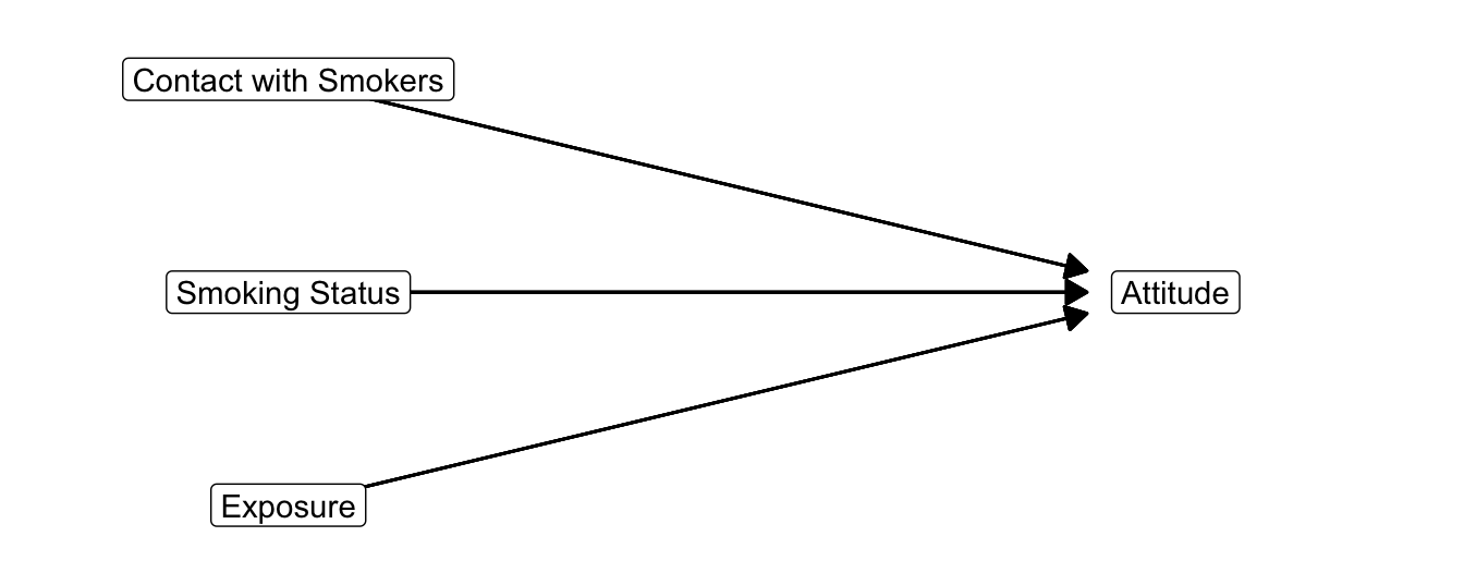
Figure 6.3: A conceptual model with some hypothesized causes of attitude towards smoking.
Figure 6.3 summarizes some hypothesized causes of the attitude towards smoking. Attitude towards smoking is measured as a scale, so it is a numerical variable. In linear regression, the dependent variable (\(y\)) must be numerical and in principle continuous. There are regression models for other types of dependent variables, for instance, logistic regression for a dichotomous (0/1) dependent variable and Poisson regression for a count dependent variable, but we will not discuss these models.
A regression model translates this conceptual diagram into a statistical model. The statistical regression model is a mathematical function with the dependent variable (also known as the outcome variable, usually referred to with the letter \(y\)) as the sum of a constant, the effects (\(b\)) of independent variables or predictors (\(x\)), which are predictive effects, and an error term (\(e\)), which is also called the residuals, see Equation (6.1).
\[\begin{equation} \small y = constant + b_1*x_1 + b_2*x_2 + b_3*x_3 + e \tag{6.1} \normalsize \end{equation}\]If we want to predict the dependent variable (\(y\)), we ignore the error term (\(e\)) in the equation. The equation without the error term [Eq. (6.2)] represents the regression line that we visualize and interpret in the following subsections. We use the error term only when we discuss the assumptions for statistical inference on a regression model in Section 6.1.4.
\[\begin{equation} \small y = constant + b_1*x_1 + b_2*x_2 + b_3*x_3 \tag{6.2} \normalsize \end{equation}\]6.1.1 A numerical predictor
Let us first have a close look at a simple regression equation, that is, a regression equation with just one predictor (\(x\)). Let us try to predict attitude towards smoking from exposure to an anti-smoking campaign.
Figure 6.4: Predicting attitude towards smoking from exposure to an anti-smoking campaign. The orange dot represents the predicted attitude for the selected value of exposure.
Good understanding of the regression equation is necessary for understanding moderation in regression models. So let us have a close look at an example equation [Eq. (6.3)]. In this example, the dependent variable attitude towards smoking is predicted from a constant and one independent variable, namely exposure to an anti-smoking campaign.
\[\begin{equation} \small attitude = constant + b*exposure \tag{6.3} \normalsize \end{equation}\]The constant is the predicted attitude if a person scores zero on all independent variables. To see this, plug in (replace) zero for the predictor in the equation (Eq. (6.4)) and remember that zero times something yields zero. This reduces the equation to the constant.
\[\begin{equation} \small \begin{split} attitude &= constant + b*0 \\ attitude &= constant + 0 \\ attitude &= constant \end{split} \tag{6.4} \normalsize \end{equation}\]For all persons scoring zero on exposure, the predicted attitude equals the value of the regression constant. This interpretation only makes sense if the predictor can be zero. If, for example, exposure had been measured on a scale ranging from one to seven, nobody can have zero exposure, so the constant has no straightforward meaning.
The unstandardized regression coefficient \(b\) represents the predicted difference in the dependent variable for a difference of one unit in the independent variable. For example, plug in the values 1 and 0 for the exposure variable in the equation. If we take the difference of the two equations, we are left with \(b\). Other terms in the two equations cancel out.
\[\begin{equation} \small \begin{split} attitude = constant + b*1 \\ \underline{- \mspace{20mu} attitude = constant + b*0} \\ attitude \mspace{4mu} difference = b*1 - b*0 = b - 0 = b \end{split} \tag{6.5} \normalsize \end{equation}\]The unstandardized regression coefficient \(b\) represents the predicted difference in the dependent variable for a difference of one unit in the independent variable.
It is the slope of the regression line.Whether this predicted difference is small or large depends on the practical context. Is the predicted decrease in attitude towards smoking worth the effort of the campaign? In the example shown in Figure 6.4, one additional unit of exposure decreases the predicted attitude by 0.6. This seems to be quite a substantial change on a scale from -5 to 5.
In the data, the smallest exposure score is (about) zero, predicting a positive attitude of 1.6. The largest observed exposure score is around eight, predicting a negative attitude of -3.2. If exposure causes the predicted differences in attitude, the campaign would have interesting effects. It may change a positive attitude into a rather strong negative attitude.
If we want to apply a rule of thumb for the strength of the effect, we usually look at the standardized regression coefficient (\(b^*\) according to APA, Beta in SPSS output). See Section 4.2.8.2 for some rules of thumb for effect size interpretation.
Note that the regression coefficient is calculated for predictor values that occur within the data set. For example, if the observed exposure scores are within the range zero to eight, these values are used to predict attitude towards smoking.
We cannot see this in the regression equation, which allows us to plug in -10, 10, or 100 as exposure values. But the values for attitude that we predict from these exposure values are probably nonsensical (if possible at all: -10 exposure?) Our data do not tell us anything about the relation between exposure and anti-smoking attitude for predictor values outside the observed zero to eight range. We should not pretend to know the effects of exposure levels outside this range. It is good practice to check the actual range of predictor values.
6.1.2 Dichotomous predictors
Instead of a numerical independent variable, we can use a dichotomy as an independent variable in a regression model. The dichotomy is preferably coded as 1 versus 0, for example, 1 for smokers and 0 for non-smokers among our respondents.
Figure 6.5: What is the difference in attitude between non-smokers and smokers?
The interpretation of the effect of a dichotomous independent variable in a regression model is quite different from the interpretation of a numerical independent variable’s effect.
It does not make sense to interpret the unstandardized regression coefficient of, for example, smoking status as predicted difference in attitude for a difference of one ‘more’ smoking status. After all, the 0 and 1 scores do not mean that there is one unit ‘more’ smoking. Instead, the coefficient indicates that we are dealing with different groups: smokers versus non-smokers.
If smoking status is coded as smoker (1) versus non-smoker (0), we effectively have two versions of the regression equation. The first equation (6.6) represents all smokers, so their smoking status score is 1. The smoking status of this group has a fixed contribution to the predicted average attitude, namely \(b\).
\[\begin{equation} \small \begin{split} attitude &= constant + b*status \\ attitude_{smokers} &= constant + b*1 \\ attitude_{smokers} &= constant + b \end{split} \tag{6.6} \normalsize \end{equation}\]Regression equation (6.7) represents all non-smokers. Their smoking status score is 0, so the smoking status effect drops from the model.
\[\begin{equation} \small \begin{split} attitude &= constant + b*status \\ attitude_{non-smokers} &= constant + b*0 \\ attitude_{non-smokers} &= constant + 0 \end{split} \tag{6.7} \normalsize \end{equation}\]If you compare the final equations for smokers [Eq. (6.6)] and non-smokers [Eq. (6.7)], the only difference is \(b\), which is present for smokers but absent for non-smokers. It is the difference between the average score on the dependent variable (attitude) for smokers and the average score for non-smokers. We are testing a mean difference. Actually, this is exactly the same as an independent-samples t test!
Imagine that \(b\) equals 1.6. This indicates that the average attitude towards smoking among smokers (coded ‘1’) is 1.6 units above the average attitude among non-smokers (coded ‘0’). Is this a small or large effect? In the case of a dichotomous independent variable, we should not use the standardized regression coefficient to evaluate effect size. The standardized coefficient depends on the distribution of 1s and 0s, that is, which part of the respondents are smokers. But this should be irrelevant to the size of the effect.
Therefore, it is recommended to interpret only the unstandardized regression coefficient for a dichotomous independent variable. Interpret it as the difference in average scores for two groups.
6.1.3 A categorical independent variable and dummy variables
How about a categorical variable containing three or more groups, for example, the distinction between respondents who smoke (smokers), stopped smoking (former smokers), and respondents who never smoked (non-smokers)? Can we include a categorical variable as an independent variable in a regression model? Yes, we can but we need a trick.
Figure 6.6: What are the predictive effects of smoking status?
In this example, smoking status is measured with three categories: (1) non-smokers, (2) former smokers, and (3) smokers. Let us use the term categorical variable only for variables containing three or more categories or groups. This makes it easy to distinguish them from dichotomous variables. This distinction is important because we can include a dichotomous variable straight away as a predictor in a regression model but we cannot do so for a variable with more than two categories. We can only include such a categorical independent variable if we change it into a set of dichotomies.
We can create a new dichotomous variable for each group, indicating whether (score 1) or not (score 0) the respondent belongs to this group. In the example, we could create the variables neversmoked, smokesnomore, and smoking. Every respondent would score 1 on one of the three variables and 0 on the other two variables (Table 6.1). These variables are called dummy variables or indicator variables.
| Original categorical variable: | neversmoked | smokesnomore | smoking |
|---|---|---|---|
| 1 - Non-smoker | 1 | 0 | 0 |
| 2 - Former smoker | 0 | 1 | 0 |
| 3 - Smoker | 0 | 0 | 1 |
If we want to include a categorical independent variable in a regression model, we must use all dummy variables as independent variables except one. In the example, we must include two out of the three dummy variables. Equation (6.8) includes dummy variables for former smokers (\(smokesnomore\)) and smokers (\(smoking\)).
Include dummy variables as independent variables for all except one categories of a categorical variable.
The category without dummy variable is the reference group.The two dummy variables give us three different regression equations: one for each smoking status category. Just plug in the correct 0 or 1 values for respondents with a particular smoking status.
Let us first create the equation for non-smokers. To this end, we replace both \(smokesnomore\) and \(smoking\) by 0. As a result, both dummy variables drop from the equation [Eq. (6.9)], so the constant is the predicted attitude for non-smokers. The non-smokers are our reference group because they are not represented by a dummy variable in the equation.
\[\begin{equation} \small \begin{split} attitude &= constant + b_1*smokesnomore + b_2*smoking \\ attitude_{non-smokers} &= constant + b_1*0 + b_2*0 \\ attitude_{non-smokers} &= constant \end{split} \tag{6.9} \normalsize \end{equation}\]For former smokers, we plug in 1 for \(smokesnomore\) and 0 for \(smoking\). The predicted attitude for former smokers equals the constant plus the unstandardized regression coefficient for the \(smokesnomore\) dummy variable (\(b_1\)), see Equation (6.10). Remember that the constant represents the non-smokers (reference group), so the unstandardized regression coefficient \(b_1\) for the \(smokesnomore\) dummy variable shows us the difference between former smokers and non-smokers: How much more positive or more negative the average attitude towards smoking is among former smokers than among non-smokers.
\[\begin{equation} \small \begin{split} attitude &= constant + b_1*smokesnomore + b_2*smoking \\ attitude_{former smokers} &= constant + b_1*1 + b_2*0 \\ attitude_{former smokers} &= constant + b_1 \end{split} \tag{6.10} \normalsize \end{equation}\]Finally, for smokers, we plug in 0 for \(smokesnomore\) and 1 for \(smoking\) [Eq. (6.11)]. The predicted attitude for smokers equals the constant plus the unstandardized regression coefficient for the \(smoking\) dummy variable (\(b_2\)). This regression coefficient, then, represents the difference in average attitude between smokers and non-smokers (reference group).
\[\begin{equation} \small \begin{split} attitude &= constant + b_1*smokesnomore + b_2*smoking \\ attitude_{smokers} &= constant + b_1*0 + b_2*1 \\ attitude_{smokers} &= constant + b_2 \end{split} \tag{6.11} \normalsize \end{equation}\]The interpretation of the effects (regression coefficients) for the included dummies is similar to the interpretation for a single dichotomous independent variable such as smoker versus non-smoker. It is the difference between the average score of the group coded 1 on the dummy variable and the average score of the reference group on the dependent variable. The reference group is the group scoring 0 on all dummy variables that represent the categorical independent variable.
If we exclude the dummy variable for the respondents who never smoked, as in the above example, the regression weight of the dummy variable \(smokesnomore\) gives the average difference between former smokers and non-smokers. If the regression weight is negative, for instance -0.8, former smokers have on average a more negative attitude towards smoking than non-smokers. If the difference is positive, former smokers have on average a more positive attitude towards smoking.
Which group should we use as reference category, that is, which group should not be represented by a dummy variable in the regression model? This is hard to say in general. If one group is of greatest interest to us, we could use this as the reference group, so all dummy variable effects express differences with this group. Alternatively, if we expect a particular ranking of the average scores, we may pick the group at the highest, lowest or middle rank as the reference group. If you can’t decide, run the regression model several times with a different reference group.
Finally, note that we should not include all three dummy variables in the regression model [Eq. (6.8)]. We can already identify the non-smokers, because they score 0 on both the \(smokesnomore\) and \(smoking\) dummy variables. Adding the \(neversmoked\) dummy variable to the regression model is like including the same independent variable twice. How can the estimation process decide which of the two identical independent variable is responsible for the effect? It can’t decide, so the estimation process fails or it drops one of the dummy variables. If this happens, the independent variables are said to be perfectly multicollinear.
6.1.4 Sampling distributions and assumptions
If we are working with a random sample or we have other reasons to believe that our data could have been different due to chance (Section 4.7.4), we should not just interpret the results for the data set that we collected. We should apply statistical inference—confidence intervals and significance tests—to our results. The confidence interval gives us bounds for plausible population values of the unstandardized regression coefficient. The p value is used to test the null hypothesis that the unstandardized regression coefficient is zero in the population.
Each regression coefficient as well as the constant may vary from sample to sample drawn from the same population, so we should devise a sampling distribution for each of them. These sampling distributions happen to have a t distribution under particular assumptions.
Chapters 3 and 4 have extensively discussed how confidence intervals and p values are constructed and how they must be interpreted. So we focus now on the assumptions under which the t distribution is a good approximation of the sampling distribution of a regression coefficient.
6.1.4.1 Independent observations
The two most important assumptions require that the observations are independent and identically distributed. These requirements arise from probability theory. If they are violated, the statistical results should not be trusted.
Each observation, for instance, a measurement on a respondent, must be independent of all other observations. A respondent’s dependent variable score is not allowed to depend on scores of other respondents.
It is hardly possible to check that our observations are independent. We usually have to assume that this is the case. But there are situations in which we should not make this assumption. In time series data, for example, the daily amount of political news, we usually have trends, cyclic movements, or issues that affect the amount of news over a period of time. As a consequence, the amount and contents of political news on one day may depend on the amount and contents of political news on the preceding days.
Clustered data should also not be considered as independent observations. Think, for instance, of student evaluations of statistics tutorials. Students in the same tutorial group are likely to give similar evaluations because they had the same tutor and because of group processes: Both enthusiasm and dissatisfaction can be contagious.
6.1.4.2 Identically distributed observations
To check the assumption of identically distributed observations, we inspect the residuals. Remember, the residuals are represented by the error term (\(e\)) in the regression equation. They are the difference between the scores that we observe for our respondents and the scores that we predict for them with our regression model.
Figure 6.7: What are the residuals and how are they distributed?
If we sample from a population where attitude towards smoking depends on exposure, smoking status, and contact with smokers, we will be able to predict attitude from the independent variables in our sample. Our predictions will not be perfect, sometimes too high and sometimes too low. The differences between predicted and observed attitude scores are the residuals.
If our sample is truly a random sample with independent and identically distributed observations, the sizes of our errors (residuals) should be normally distributed for each value of the dependent variable, that is, attitude in our example. The residuals should result from chance for the relation between chance and a normal distribution).
So for all possible values of the dependent variable, we must collect the residuals for the observations that have this score on the dependent variable. For example, we should select all respondents who score 4.5 on the attitude towards smoking scale. Then, we select the residuals for these respondents and see whether they are approximately normally distributed.
Usually, we do not have more than one observation (if any) for a single dependent variable score, so we cannot apply this check. Instead, we use a simple and coarse approach: Are all residuals normally distributed?
A histogram with an added normal curve (like the right-hand plot in Figure 6.7) helps us to evaluate the distribution of the residuals. If the curve more or less follows the histogram, we conclude that the assumption of identically distributed observations is plausible. If not, we conclude that the assumption is not plausible and we warn the reader that the results can be biased.
6.1.4.3 Linearity and prediction errors
The other two assumptions that we use tell us about problems in our model rather than problems in our statistical inferences. Our regression model assumes a linear effect of the independent variables on the dependent variable (linearity) and it assumes that we can predict the dependent variable equally well or equally badly for all levels of the dependent variable (homoscedasticity, next section).
The regression models that we estimate assume a linear model. This means that an additional unit of the independent variable always increases or decreases the predicted value by the same amount. If our regression coefficient for the effect of exposure on attitude is -0.25, an exposure score of one predicts a 0.25 more negative attitude towards smoking than zero exposure. Exposure score five predicts the same difference in comparison to score four as exposure score ten in comparison to exposure score nine, and so on. Because of the linearity assumption, we can draw a regression model as a straight line. Residuals of the regression model help us to see whether the assumption of a linear effect is plausible.
Figure 6.8: How do residuals tell us whether the relation is linear?
The relation between an independent and dependent variable, for example, exposure and attitude towards smoking, does not have to be linear. It can be curved or have some other fancy shape. Then, the linearity assumption is not met. A straight regression line does not nicely fit such data.
We can see this in a graph showing the (standardized) residuals (vertical axis) against the (standardized) predicted values of the dependent variable (on the horizontal axis), as exemplified by the lower plot in Figure 6.8. Note that the residuals represent prediction errors. If our regression predictions are systematically too low at some levels of the dependent variable and too high at other levels, the residuals are not nicely distributed around zero for all predicted levels of the dependent variable. This is what you see if the association is curved or U-shaped.
This indicates that our linear model does not fit the data. If it would fit, the average prediction error is zero for all predicted levels of the dependent variable. Graphically speaking, our linear model matches the data if positive prediction errors (residuals) are more or less balanced by negative prediction errors everywhere along the regression line.
6.1.4.4 Homoscedasticity and prediction errors
The plot of residuals by predicted values of the dependent variable tells us more than whether a linear model fits the data.
Figure 6.9: How do residuals tell us that we predict all values equally well?
The other assumption states that we can predict the dependent variable equally well at all dependent variable levels. In other words, the prediction errors (residuals) are more or less the same at all levels of the dependent variable. This is called homoscedasticity. If we have large prediction errors at some levels of the dependent variable, we should also have large prediction errors at other levels. As a result, the vertical width of the residuals by predictions scatter plot should be more or less the same from left to right. The dots representing residuals resemble a more or less rectangular band.
If the prediction errors are not more or less equal for all levels of the predicted scores, our model is better at predicting some values than other values. For example, low values can be predicted better than high values of the dependent variable. The dots representing residuals resemble a cone. This may signal, among other things, that we need to include moderation in the model.