Chapter 7 Regression Analysis With A Numerical Moderator
Key concepts: interaction variable, common support, simple slope, conditional effect, mean-centering.
Watch this micro lecture on regression models with a numerical moderator for an overview of the chapter.
Summary
Chapter 6 shows us how we can include dichotomous and categorical variables as predictors and moderators in a regression model. Using dummy variables, we can analyze mean differences between groups and we can construct different regression lines for different groups (moderation). A graph showing the different regression models for different moderator groups communicates the results of a moderation model in an attractive way.
What if our moderator is not dichotomous or categorical but numerical? For example, the effect of exposure to an anti-smoking campaign on attitude towards smoking can be different for people of different age or for people who spend more time with smokers.
We can include a numerical moderator in a regression model just like a dichotomous moderator. Add the predictor, the moderator, and an interaction variable, which is the product of the moderator and the predictor. If both the predictor and moderator are numerical, the interaction variable is numerical. It gives us numbers, not groups.
The interpretation of an interaction effect is different if the moderator is numerical instead of dichotomous or categorical. In general, the regression coefficient of a numerical variable expresses the effect of a one unit change. For a numerical predictor, this is the predicted change in the dependent variable. For a numerical moderator, however, it is the predicted change in the effect of the predictor. The unstandardized regression coefficient for a numerical moderator, then, tells us the predicted change in the effect of the predictor for a one unit increase in the moderator.
This interpretation is quite abstract and not easy to understand. It is better to visualize the regression lines for different values of the moderator. We usually draw regression lines for three interesting moderator values. The mean value of the moderator shows us the effect at a medium level of the moderator. One standard deviation below or above the mean of the moderator represent attractive low and high moderator values.
Just like a model with a dichotomous or categorical moderator, the effect of a predictor that is involved in moderation is a conditional effect. In other words, it is the effect of that predictor conditioned under one particular value of the moderator, namely the value zero. Unfortunately, zero is not always a meaningful value for the moderator. If it does not exist or appears rarely on the moderator, it is better to mean-center the moderator. Mean-centering a variable changes the scores such that the mean of the original variable becomes zero on the mean-centered variable. The value zero is always meaningful for a mean-centered variable because it represents the mean score on the original variable. With a mean-centered moderator, the regression coefficient of the predictor always makes sense.
Essential Analytics
As in Chapter 6, we calculate an interaction variable as the product of the predictor and moderator (the Compute Variable option in the Transform menu) and we use it as one of the independent variables in a linear regression model (the Linear option in the Regression submenu).
The regression coefficient of the predictor tells us how much the predicted value of the dependent variable changes for a one unit increase in the predictor score for cases that score zero on the moderator. For example, one additional unit of exposure to the campaign decreases the attitude towards smoking by (-)0.53 for people with zero contacts with smokers (Figure 7.1, red box). The cases that score zero on the moderator (here: people with zero contacts with smokers) are the reference group; zero is the reference value.
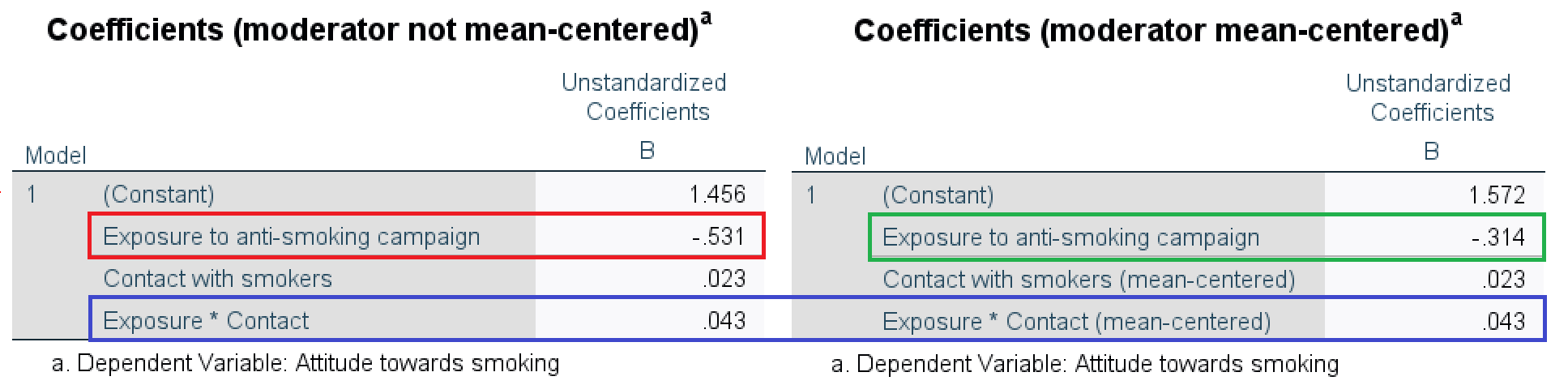
Figure 7.1: SPSS table of regression effects for a model in which the effect of exposure is moderated by contact with smokers: with the original variables (left) and with the moderator mean-centered (right).
It is wise to mean-center the moderator variable before we use it. To mean-center a variable, we first obtain the value of the variable’s mean with the Statistics option in the Frequencies submenu of Descriptive Statistics. Next, we use the Compute Variable option in the Transform menu to subtract this mean from the original variable.
The effect of exposure on attitude changes if we mean-center the moderator variable contact (Figure 7.1, green box). People with an average number of contacts with smokers score zero on the mean-centered variable, so they are the new reference group. Among people with an average number of contacts with smokers, one additional unit of exposure decreases the predicted attitude by (-)0.31.
The regression coefficient of the interaction effect (Figure 7.1, blue box) tells us how much the effect of the predictor changes if the moderator increases by one unit. One additional contact with a smoker increases the effect of exposure on attitude by 0.04, making it 0.04 less strongly negative or more strongly positive.
Communicate the results of a numerical moderator in a scatterplot (Scatter/Dot in the Legacy Dialogs submenu of the Graphs menu) with regression lines for the effect of the predictor at three moderator values: the mean value of the moderator, one standard deviation below the mean and one standard deviation above the mean (Figure 7.2). Get the mean and standard deviation of the moderator variable with the Statistics option in the Frequencies submenu of Descriptive Statistics and plug these values in the regression equation along with suitable values of any covariates. Add the resulting (simple) regression equations to the scatterplot with the Reference Line from Equation option in the Options menu of the Chart Editor.
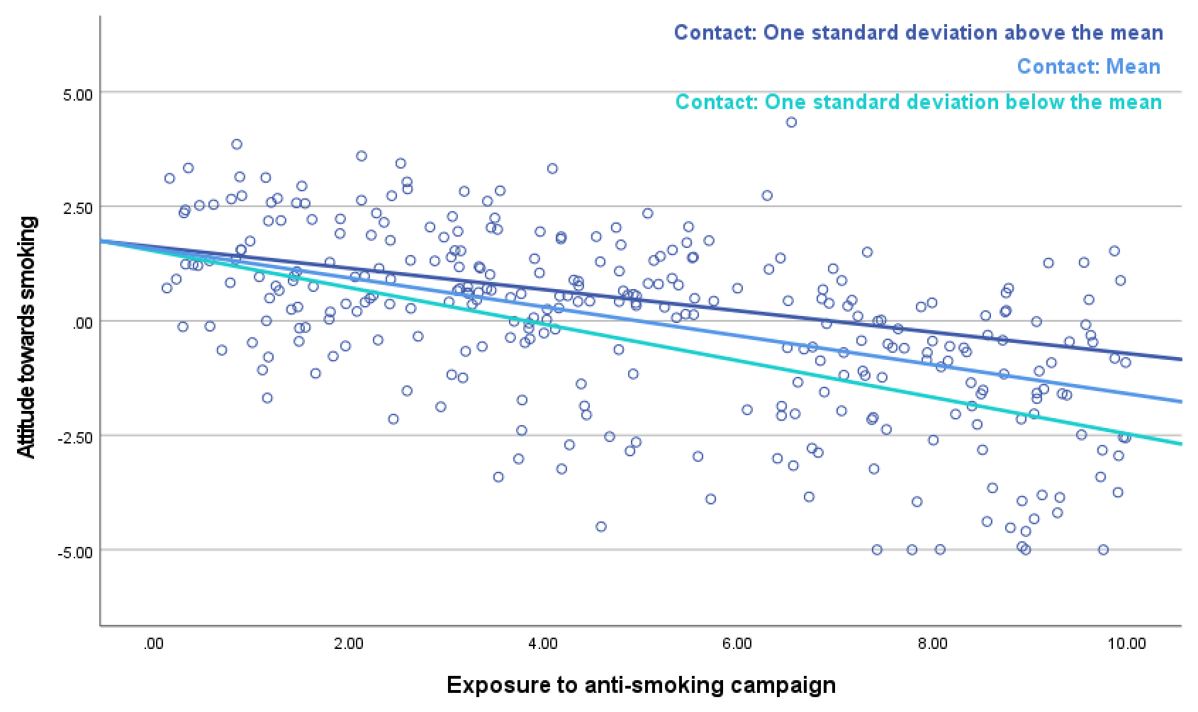
Figure 7.2: Plot of the effect of exposure on attitude towards smoking for three levels of the moderator variable: contact with smokers.