4.5 Confidence Intervals to test hypotheses
In Chapter 3, we learned how to calculate a confidence interval for the population mean. We also learned that the confidence interval is a range of values that is likely to contain the true population mean. We learned that the true population mean falls within the confidence in 95% of a hundred samples. We can use this knowledge to test hypotheses. If we, again, have the hypothesis that the average media literacy in the population is 5.5, we can use the confidence interval to test this hypothesis. If we draw a sample and calculate the confidence interval, we can see if the hypothesized population mean falls within the confidence interval. If it does, we can conclude that we are probably right. If it does not, we can conclude that we are probably wrong.
With the hypothesis that we can improve media literacy through some intervention program, we can also use the confidence interval to test this hypothesis. If the lower bound of the confidence interval is higher than 5.5, we can conclude that the intervention program works.
4.5.1 Estimation in addidion to NHST
Following up on a report commissioned by the American Psychological Association APA (Wilkinson, 1999), the 6th edition of the Publication Manual of the American Psychological Association recommends reporting and interpreting confidence intervals in addition to null hypothesis significance testing.
Estimation is becoming more important: Assessing the precision of our statements about the population rather than just rejecting or not rejecting our hypothesis about the population. This is an important step forward and it is easy to accomplish with your statistical software.
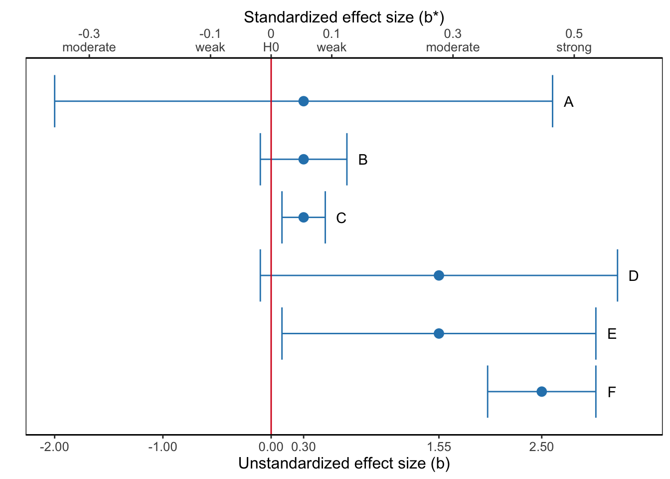
Figure 4.19: What is the most sensible interpretation of the results represented by the confidence interval for the regression coefficient, which estimates brand awareness from campaign exposure?
Figure 4.19 shows six confidence intervals for a population value, for instance, the effect of exposure to advertisements on brand awareness, and the sample result as point estimate (dot). The horizontal axis is labeled by the size of the effect: the difference between the effect in the sample and the absence of an effect according to the null hypothesis.
A confidence interval shows us whether or not our null hypothesis must be rejected. The rule is simple: If the value of the null hypothesis is within the confidence interval, the null hypothesis must not be rejected. By the way, note that a confidence interval allows us to test a null hypothesis other than the nil (Section 3.5.1). If we hypothesize that the effect of exposure on brand awareness is 0.1, we reject this null hypothesis if the confidence interval of the regression coefficient does not include 0.1. SPSS usually tests nil hypotheses, this can be adjusted for some tests, but not all. Though it is almost always possible to visualize the confidence interval in graphs created in SPSS.
Confidence intervals allow us to draw a more nuanced conclusion. A confidence interval displays our uncertainty about the result. If the confidence interval is wide, we are quite uncertain about the true population value. If a wide confidence interval includes the null hypothesis, but the value specified in the null hypothesis is located near one of its boundaries (e.g., Confidence Interval D in Figure 4.19), we do not reject the null hypothesis. However, it still is plausible that the population value is substantially different from the hypothesized value.
For example, we could interpret Confidence Interval D in Figure 4.19 in the following way:
The effect of exposure to advertisements on brand awareness is of moderate size in the sample (b* = 0.28). It is, however, not statistically significant, t (23) = 1.62, p = .119, 95% CI [-0.1, 3.2], meaning that we are not sufficiently confident that there is a positive effect in the population. It is important to note that the sample is small (N = 25– this number is not included in the figure–), so test power is probably low, meaning that it is difficult to reject a false null hypothesis. On the basis of the confidence interval we conclude that the effect can be weak and negative, but the plausible effects are predominantly positive, including strong positive effects. One additional daily exposure may decrease predicted brand awareness by 0.1, but it may also increase brand awareness by up to 3.2 points on a scale from 1 (unaware of the brand) to 7 (highly aware of the brand). The latter effect is substantial: A single additional exposure to advertisements would lead to a substantial change in brand awareness.
We should report that the population value seems to be larger (smaller) than specified in the null hypothesis but that we do not have sufficient confidence in this result because the test is not statistically significant. This is better than reporting that there is no difference because the statistical test is not significant.
The fashion of speaking of a null hypothesis as “accepted when false”, whenever a test of significance gives us no strong reason for rejecting it, and when in fact it is in some way imperfect, shows real ignorance of the research workers’ attitude, by suggesting that in such a case he has come to an irreversible decision.
The worker’s real attitude in such a case might be, according to the circumstances:
- “The possible deviation from truth of my working hypothesis, to examine which the test is appropriate, seems not to be of sufficient magnitude to warrant any immediate modification.”
Or it might be:
- “The deviation is in the direction expected for certain influences which seemed to me not improbable, and to this extent my suspicion has been confirmed; but the body of data available so far is not by itself sufficient to demonstrate their reality.”
In a similar way, a very narrow confidence interval including the null hypothesis (e.g., Confidence Interval B in Figure 4.19) and a very narrow confidence interval near the null hypothesis but excluding it (e.g., Confidence Interval C in Figure 4.19) should not yield opposite conclusions because the statistical test is significant in the second but not in the first situation. After all, even for the significant situation, we know with high confidence (narrow confidence interval) that the population value is close to the hypothesized value.
For example, we could interpret Confidence Interval C in Figure 4.19 in the following way:
The effect of exposure to advertisements on brand awareness is statistically significant, t (273) = 3.67, p < .001, 95% CI [0.1, 0.5]. On the basis of the confidence interval we are confident that the effect is positive but small (maximum b* = 0.05). One additional daily exposure increases predicted brand awareness by 0.1 to 0.5 on a scale from 1 (unaware of the brand) to 7 (highly aware of the brand). We need a lot of additional exposure to advertisements before brand awareness changes substantially.
In addition, it is good practice to include confidence intervals in research report figures. Especially in figures depicting moderation (see Chapter 5.3.1), confidence intervals can help to interpret where differences between multiple groups are likely to occur.
Using confidence intervals in this way, we avoid the problem that statistically non-significant effects are not published. Not publishing non-significant results, either because of self-selection by the researcher or selection by journal editors and reviewers, offers a misleading view of research results.
If results are not published, they cannot be used to design new research projects. For example, effect sizes that are not statistically significant are just as helpful to determine test power and sample size as statistically significant effect sizes. An independent variable without statistically significant effect may have a significant effect in a new research project and should not be discarded if the potential effect size is so substantial that it is practically relevant. Moreover, combining results from several research projects helps making more precise estimates of population values, which brings us to meta-analysis.
4.5.2 Bootstrapped confidence intervals
Using the confidence interval is the easiest and sometimes the only way of testing a null hypothesis if we create the sampling distribution with bootstrapping. For instance, we may use the median as the preferred measure of central tendency rather than the mean if the distribution of scores is quite skewed and the sample is not very large. In this situation, a theoretical probability distribution for the sample median is not known, so we resort to bootstrapping.
Bootstrapping creates an empirical sampling distribution: a lot of samples with a median calculated for each sample. A confidence interval can be created from this sampling distribution (see Section 3.5.2). If our null hypothesis about the population median is included in the 95% confidence interval, we do not reject the null hypothesis. Otherwise, we reject it. We will encounter this in Chapter 9 about mediation, where indirect effects are tested with bootstrapped confidence intervals.