Chapter 6 Regression Analysis And A Categorical Moderator
Key concepts: regression equation, dummy variables, normally distributed residuals, linearity, homoscedasticity, independent observations, statistical diagram, interaction variable, covariate, common support, simple slope, conditional effect.
Watch this micro lecture on regression analysis with a categorical moderator for an overview of the chapter.
Summary
The linear regression model is a powerful and very popular tool for predicting a numerical dependent variable from one or more independent variables. In this chapter, we use regression analysis to evaluate the effects of an anti-smoking campaign. We predict attitude towards smoking from exposure to the anti-smoking campaign (numerical), time spent with smokers (numerical), and the respondent’s smoking status (categorical).
Regression coefficients, that is, the slopes of regression lines, are the effects in a regression model. They show the predicted difference in the dependent variable for a one unit difference in the independent variable (exposure, time spent with smokers) or the predicted mean difference for two categories (smokers versus non-smokers).
But what if the predictive effect is not the same in all contexts? For example, exposure to an anti-smoking campaign may generally generate a more negative attitude towards smoking. The effect, however, is probably different for people who smoke than for people who do not smoke. In this case, the effect of campaign exposure on attitude towards smoking is moderated by context: Whether or not the person exposed to the campaign is a smoker.
Different effect sizes for different contexts are different regression coefficients for different contexts. We need different regression lines for different groups of people. We can use an interaction variable as an independent variable in a regression model to accommodate for moderation as different effects. An interaction variable is just the product of the predictor variable and the moderator variable.
As an independent variable in the model, the regression coefficient of an interaction variable (interaction effect for short) has a confidence interval and a p value. The confidence interval tells us the plausible values for the size of the interaction effect in the population. The p value tests the null hypothesis that there is no interaction effect at all in the population.
To interpret the interaction effect, we must determine the size of the effect of the predictor on the dependent variable for each group of the moderator. For example, the effect of campaign exposure on smoking attitude for smokers and the effect for non-smokers.
An interaction effect in a regression model closely resembles an interaction effect in analysis of variance. The effect of a single predictor that is involved in an interaction effect in a regression model, however, is not a main effect as in analysis of variance. It is a conditional effect, namely the effect for one particular value of the moderator, that is, the effect within one particular context. To understand this, we must pay close attention to the regression equation.
Essential Analytics
In SPSS, we use the Linear option in the Regression submenu for regression analysis. For a moderation model, we first use the Compute Variable option in the Transform menu to calculate an interaction variable: we multiply (using *) the predictor variable by the moderator variable. The interaction variable is included in the regression model as an independent variable, just like the predictor, moderator, and any other independent variables (covariates).
A categorical predictor variable such as a participant’s residential area (urban, suburban, rural) is included in the regression model as dummy variables, which have the values 0 or 1, for example: dummy variables suburban and rural, each with values yes (1) and no (0). The category without dummy variable is the reference group.
The regression coefficient of a dummy variable gives us the difference between the average score on the dependent variable of the group scoring 1 on the dummy variable and the reference group. In the example presented in Figure 6.1, the attitude towards smoking for participants living in a suburban environment (red box) is on average 0.33 more positive than among participants in an urban environment (the reference group).
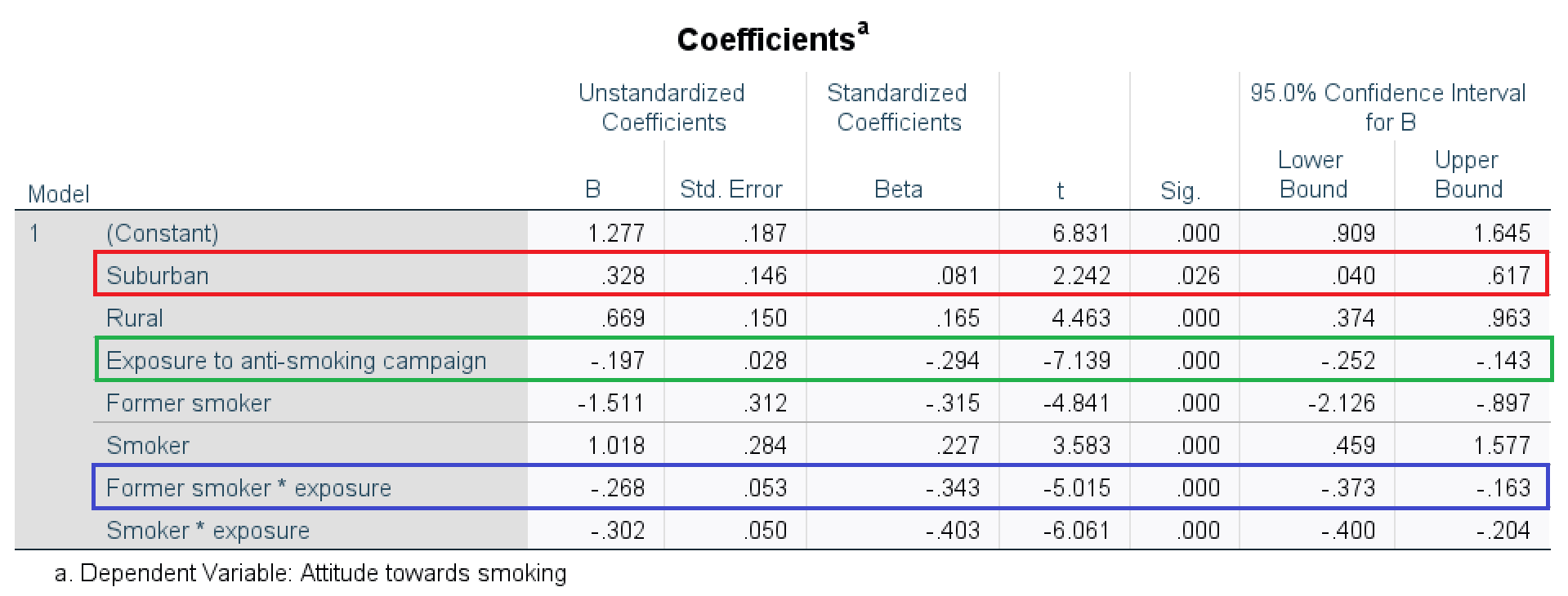
Figure 6.1: SPSS table of regression effects for a model in which the effect of exposure is moderated by participant’s smoking status (reference group: people who never smoked).
The predictor variable Exposure is included in the interaction effect. As a consequence, the regression coefficient for this variable (green box in Figure 6.1) expresses the effect of exposure on attitude towards smoking for the reference group on the other variable included in the interaction effect, namely, people who never smoked. A one unit increase in exposure predicts a 0.20 more negative (-0.197) attitude towards smoking for people who never smoked.
If we would like to know the effect of exposure on attitude towards smoking for former smokers, we must add the regression coefficient for the interaction of exposure with former smokers (blue box) to the regression coefficient of exposure (green box): A one unit increase in exposure predicts a 0.47 more negative (-0.465 = -0.197 + -0.268) attitude towards smoking for former smokers.
An interaction effect such as -0.27 for Former smoker * exposure tells us the difference between the exposure effect for former smokers and the exposure effect for people who never smoked (reference group). A plot of the regression lines shows the different exposure effects (Figure 6.2). The red line (effect of exposure for former smokers) has a stronger downward tendency than the blue line (exposure effect for people who never smoked).
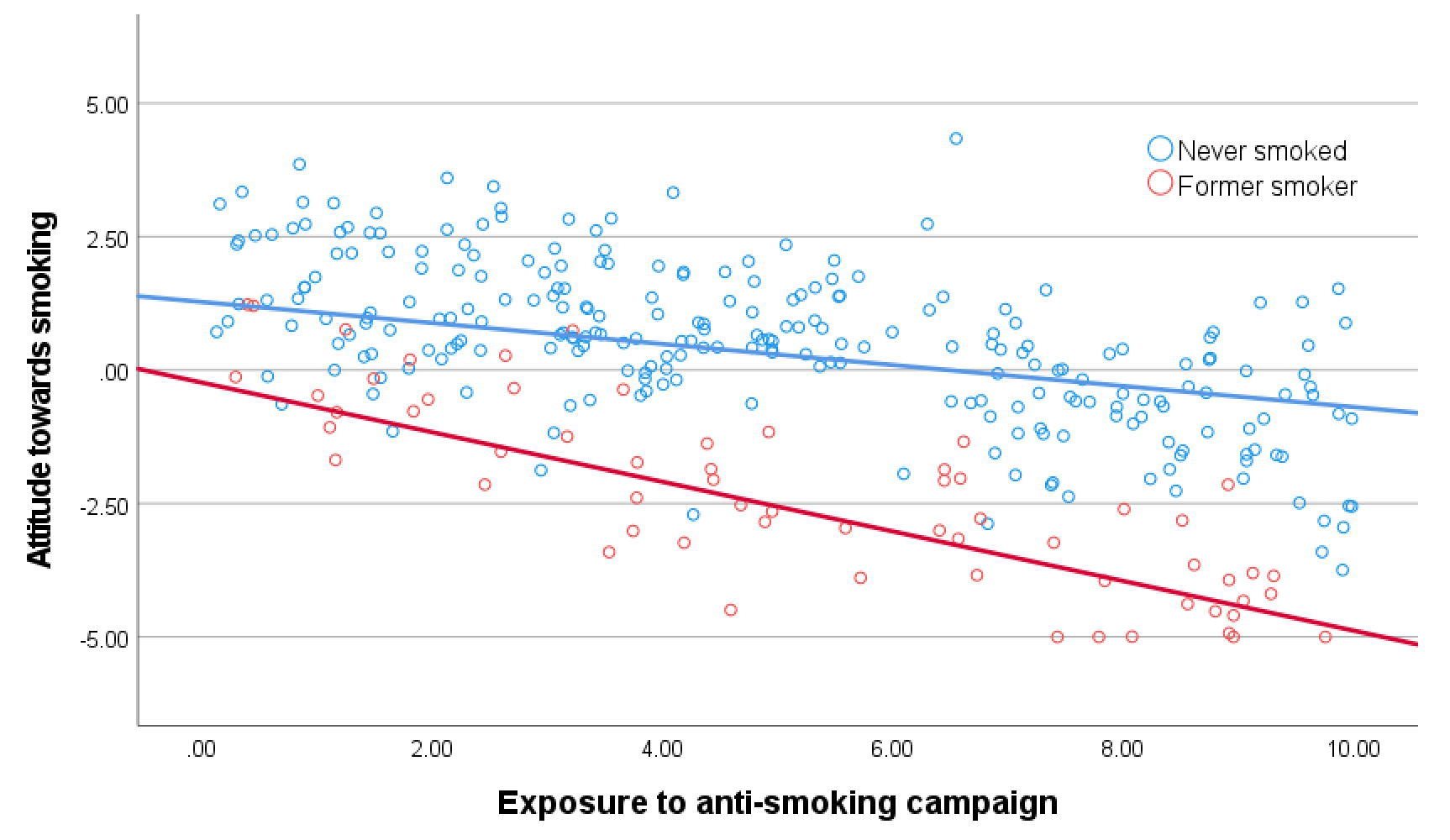
Figure 6.2: Simple regression lines showing the effect of exposure on attitude towards smoking for former smokers and people who never smoked (in an urban environment).