5.3 Different Means for Two Factors
The participants in the experiment do not only differ because they see different endorsers in the charity video. In addition, there are differences according to sex: female versus male participants. Does participant’s sex matter to the effect of the endorser on willingness to donate?
Figure 5.9: How do group means inform us about (main) effects in analysis of variance?
In the preceding section, we have looked at the effect of a single factor on willingness to donate, namely, the endorser to whom participants are exposed. Thus, we take into account two variables: one independent variable and one dependent variable. This is an example of bivariate analysis.
Usually, however, we expect an outcome to depend on more than one variable. Willingness to donate does not depend only on the celebrity endorsing a fundraising campaign. It is easy to think of more factors, such as a person’s available budget, her personal level of altruism, and so on.
It is straightforward to include more factors in an analysis of variance. These can be additional experimental treatments in the context of an experiment as well as participant characteristics that are not manipulated by the researcher. For example, we may hypothesize that females are generally more charitable than males.
5.3.1 Two-way analysis of variance
If we use one factor, the analysis is called one-way analysis of variance. With two factors, it is called two-way analysis of variance, and with three factors… well, you probably already guessed that name.
A two-way analysis of variance using a factor with three levels, for instance, exposure to three different endorsers, and a second factor with two levels, for example, female versus male, is called a 3x2 (say: three by two) factorial design.
5.3.2 Balanced design
In analysis of variance with two or more factors, it is quite nice if the factors are statistically independent from one another. In other words, it is nice if the scores on one factor are not associated with scores on another factor. This is called a balanced design.
In an experiment, we can ensure that factors are independent if we have the same number of participants in each combination of levels on all factors. In other words, a factorial design is balanced if we have the same number of observations in each subgroup. A subgroup contains the participants that have the same level on both factors just like a cell in a contingency table.
| Female | Male | |
|---|---|---|
| Clooney | 2 | 2 |
| Jolie | 2 | 2 |
| No endorser | 2 | 2 |
Table 5.1 shows an example of a balanced 3x2 factorial design. Each subgroup (cell) contains two participants (cases). Equal distributions of frequencies across columns or across rows indicate statistical independence. In the example, the distributions are the same across columns (and rows), so the factors are statistically independent.
In practice, it may not always be possible to have exactly the same number of observations for each subgroup. A participant may drop out from the experiment, a measurement may go wrong, and so on. If the numbers of observations are more or less the same for all subgroups, the factors are nearly independent, which is okay. We can use the same rule of thumb for a balanced design as for the conditions of an F test in analysis of variance: If the size of the smallest subgroup is less than ten per cent smaller than the size of the largest group, we call a factorial design balanced.
A balanced design is nice but not necessary. Unbalanced designs can be analyzed but estimation is more complicated (a problem for the computer, not for us) and the assumption of equal population variances for all groups (Levene’s F test) is more important (a problem for us, not for the computer) because we do not have equal group sizes. Note that the requirement of equal group sizes applies to the subgroups in a two-way analysis of variance. With a balanced design, we ensure that we have the same number of observations in all subgroups, so we are on the safe side.
5.3.3 Main effects in two-way analysis of variance
A two-way analysis of variance tests the effects of both factors on the dependent variable in one go. It tests the null hypothesis that participants exposed to Clooney have the same average willingness to donate in the population as participants exposed to Jolie or those who are not exposed to an endorser. At the same time, it tests the null hypothesis that females and males have the same average willingness to donate in the population.
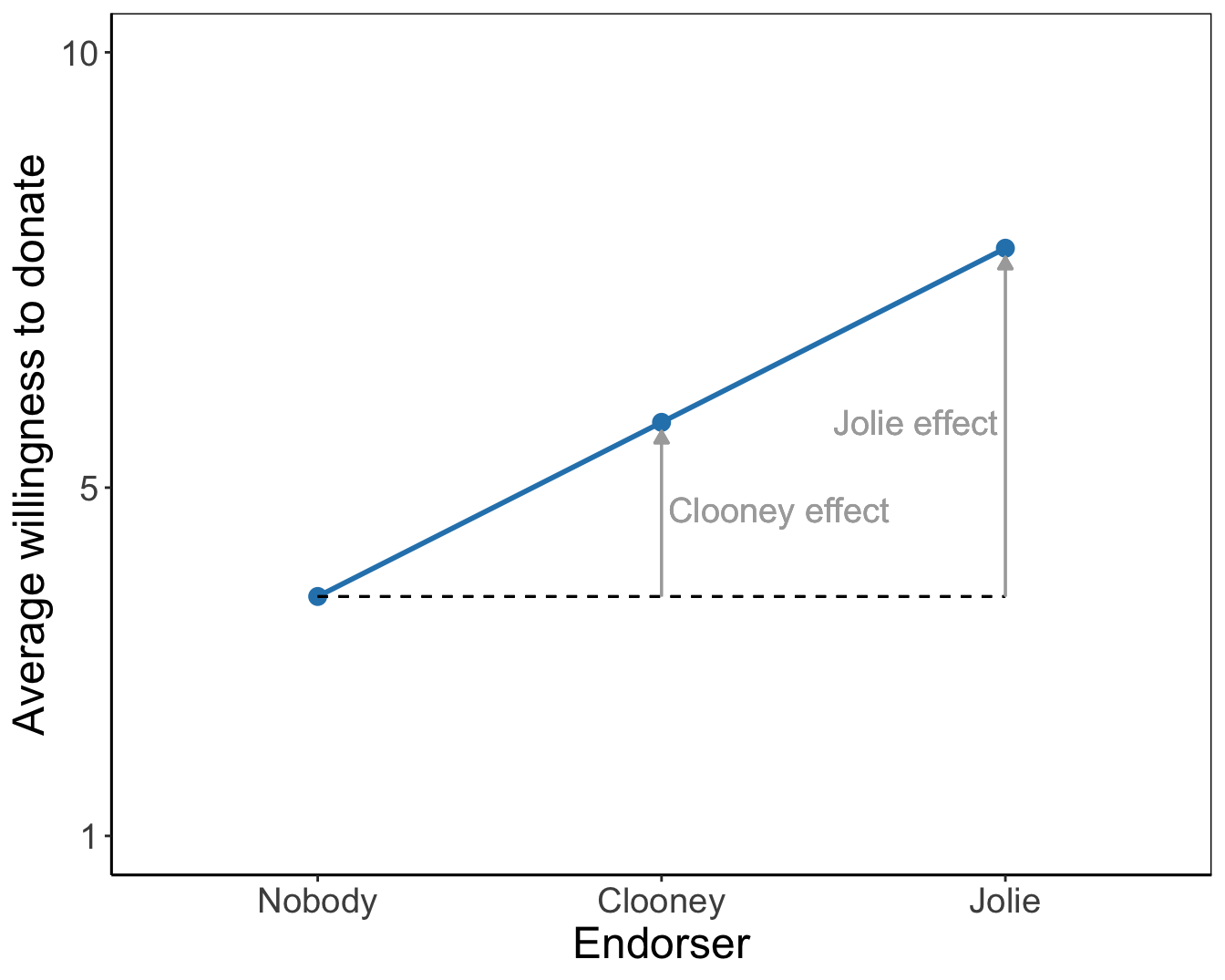
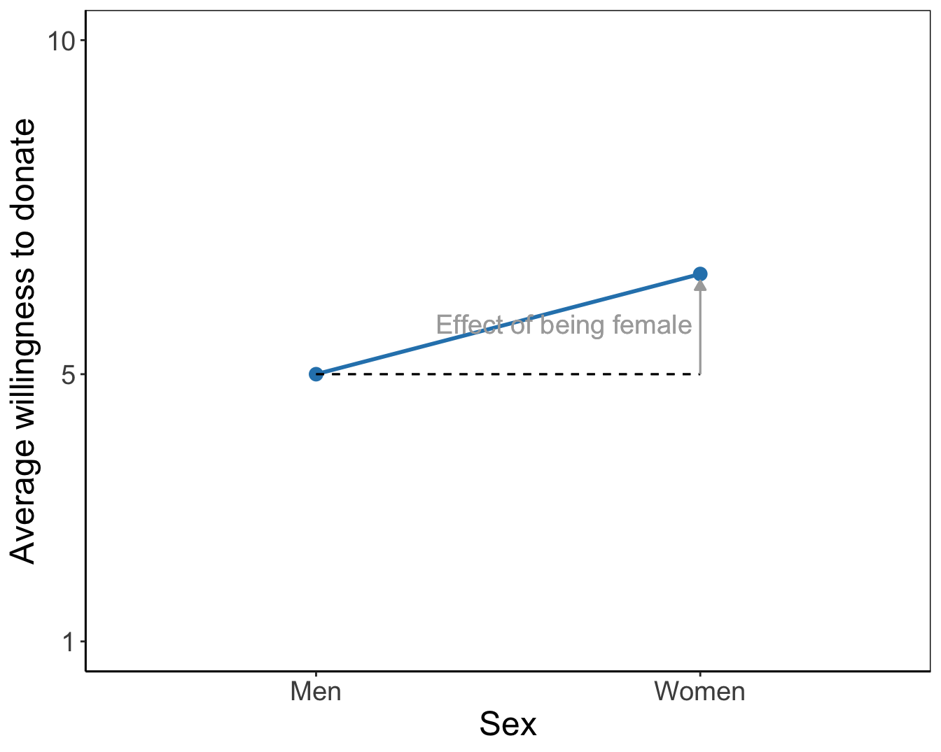
Figure 5.10: Means plots for the main effects of endorser and sex on willingness to donate. As a reading instruction, effects of endorsers and of being female are represented by arrows.
The tested effects are main effects because they represent the effect of one factor. They express an overall or average difference between the mean scores of the groups on the dependent variable. The main effect of the endorser factor shows the mean differences for endorser groups if we do not distinguish between females and males. Likewise, the main effect for sex shows the average difference in willingness to donate between females and males without taking into account the endorser to whom they were exposed.
We could have used two separate one-way analyses of variance to test the same effects. Moreover, we could have tested the difference between females and males with an independent-samples t test. The results would have been the same (if the design is balanced.) But there is an important advantage to using a two-way analysis of variance, to which we turn in the next section.