7.2 Reporting Regression Results
If we report a regression model, we first present the significance test and predictive power of the entire regression model. We may report that the regression model is statistically significant, F (7, 142) = 28.64, p < 0.001, so the regression model very likely helps to predict attitude towards smoking in the population.
How well does the regression model predict attitude towards smoking? The effect size of a regression model or its predictive power is summarized by \(R^2\) (R Square), which is the proportion of the variance in the dependent variable scores (attitude towards smoking) that can be predicted with the regression model. In this example, \(R^2\) is 0.59, so the regression model predicts 59% of the variance in attitude towards smoking among the respondents. In communication research, \(R^2\) is usually smaller.
\(R^2\) tells us how well the regression model predicts the dependent variable in the sample. Every predictor that we add to the regression model helps to predict results in the sample even if the predictor does not help to predict the dependent variable in the population. For a better idea of the predictive power of the regression model in the population, we may use Adjusted R Square. Adjusted R Square is usually slightly lower than R Square. In the example, Adjusted R Square is 0.56 (not reported in Table 7.2).
| B | 95% CI | |
|---|---|---|
| Constant | -1.08*** | [-1.32, -0.85] |
| Exposure | -0.18*** | [-0.26, -0.10] |
| Contact | 0.21*** | [ 0.12, 0.30] |
| Former smoker | -1.38*** | [-1.74, -1.01] |
| Smoker | 0.10 | [-0.41, 0.60] |
| Exposure * Contact | 0.06*** | [ 0.02, 0.09] |
| Exposure * Former smoker | -0.20** | [-0.33, -0.07] |
| Exposure * Smoker | -0.02 | [-0.17, 0.13] |
| R2 | 0.59 | |
| F (7, 142) | 28.64*** | |
| Note. N = 150. CI = confidence interval. | ||
| * p < .05. ** p < .01. *** p < .001. |
As a next step, we discuss the size, statistical significance, and confidence intervals of the regression coefficients. If a predictor is involved in one or more interaction effects, we must be very clear about the reference value or reference group to which the effect applies. In the example below, non-smokers are the reference group on the smoking status variable because they are not represented by a dummy variable. Average number of contacts with smokers is the reference value on the contact variable because this variable is mean-centered.
Exposure, in our example, has a negative predictive effect on attitude towards smoking (b = -0.18) for non-smokers with average contacts with smokers, t = -4.37, p < .001, 95% CI [-0.26, -0.10]. Note that SPSS does not report the degrees of freedom for the t test on a regression coefficient, so we cannot report them.
Instead of presenting the numerical results in the text, we may summarize them in an APA style table, such as Table 7.2. Note that t and p values are not reported in this table, the focus is on the confidence intervals. The significance level is indicated by stars.
A sizable and statistically significant interaction effect signals that an effect is moderated. In the example reported in Table 7.2, the effect of exposure on attitude seems to be moderated by contact with smokers (b = 0.06, p < .001) and by smoking status (b = -0.20, p = 0.003 for former smoker).
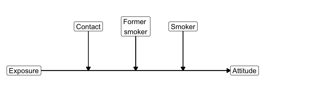
Figure 7.9: Conceptual diagram of the estimated moderation model.
The regression coefficients for interaction effects must be interpreted as effect differences. For a categorical moderator, the coefficient describes the effect size difference between the category represented by the dummy variable and the reference group. The negative effect of exposure is stronger for former smokers than for the reference group non-smokers. The average difference is -0.20.
For a numerical moderator, we can interpret the general pattern reflected by the interaction effect. A positive interaction effect, such as 0.06 for the interaction between exposure and smoker contact, signals that the effect of exposure is more strongly positive or less strongly negative at higher levels of contact with smokers.
This interpretation in terms of effect differences remains difficult to understand. It is recommended to select some interesting values for the moderator and report the size of the effect for each value. For a categorical moderator, each category is of interest. For a numerical moderator, the mean and one standard deviation below and above the mean are usually interesting values. The regression coefficients show whether the effect is positive, negative, or nearly zero at different values of the moderator.
Visualize the regression lines for different values of the moderator in addition to presenting the numerical results. If the regression model contains covariates, mention the values that you have used for the covariates. Select one of the categories for a categorical covariate. For numerical covariates, the mean is a good choice. If you are working with mean-centered predictors, be sure to use the mean-centered predictor for the horizontal axis (as in Figure 7.10), not the original predictor.
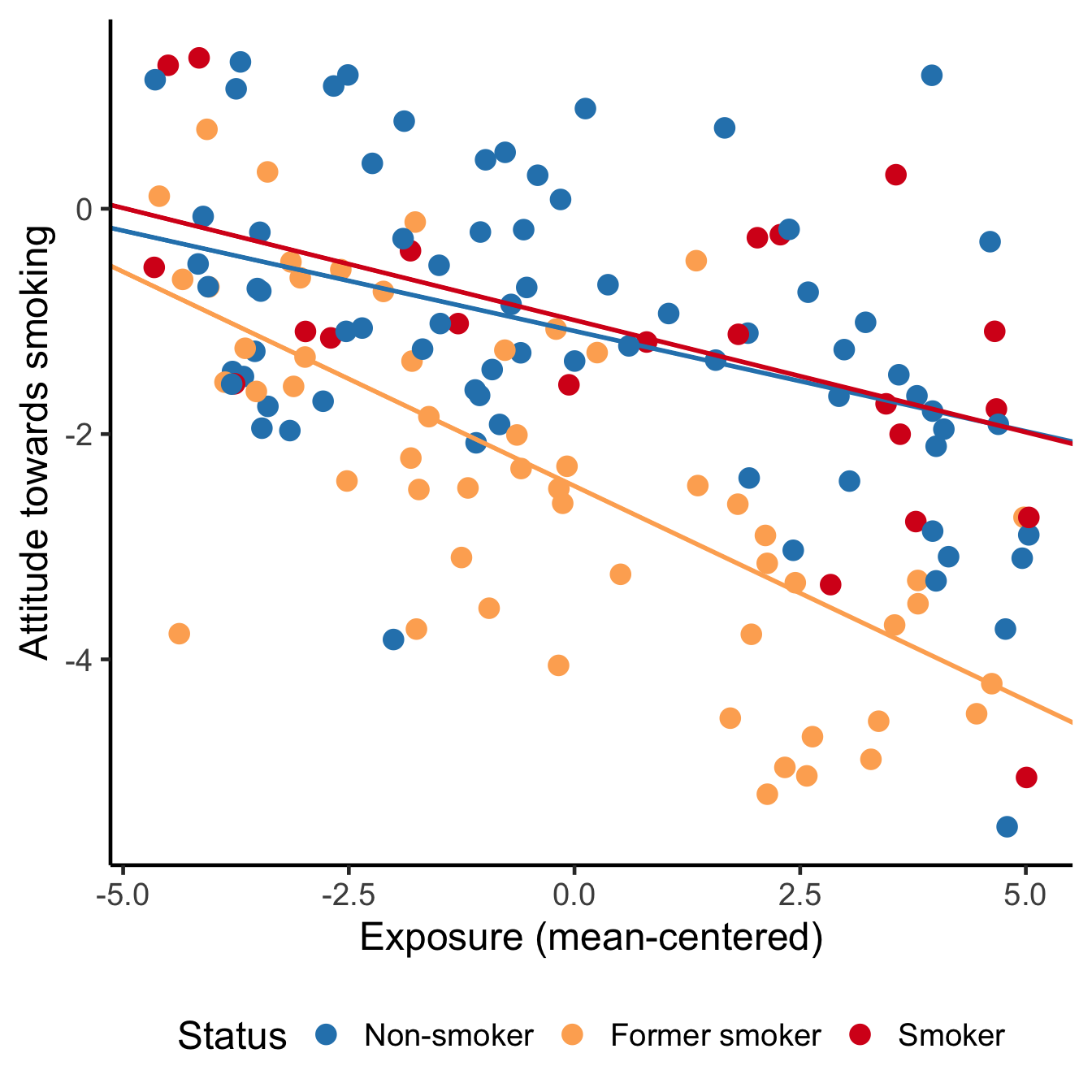
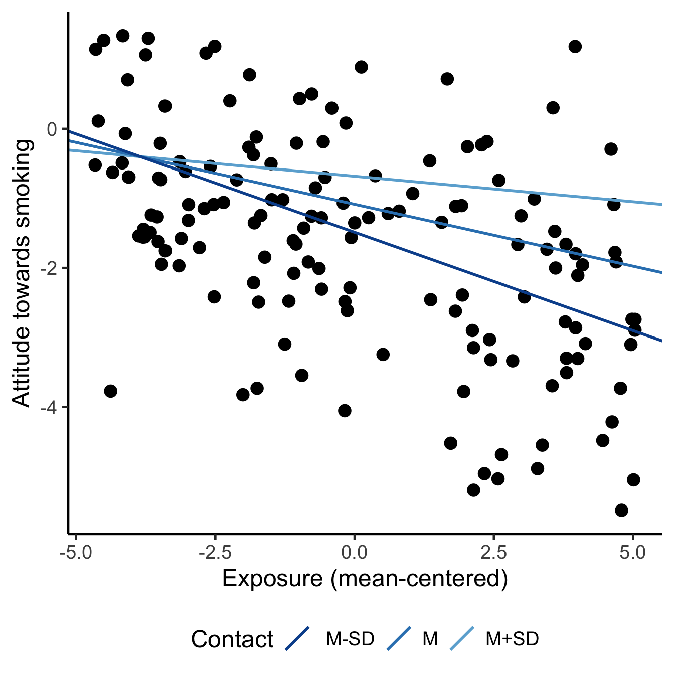
Figure 7.10: The effect of exposure on attitude towards smoking. Left: Effects for groups with different smoking status (at average contact with smokers). Right: Effects at different levels of contact with smokers (effects for non-smokers).
The left panel in Figure 7.10 clearly shows that the effect of exposure on attitude is more or less the same for non-smokers and smokers. The effect is different for former smokers, for whom the exposure effect is more strongly negative. It is more difficult to communicate this conclusion with the table of regression coefficients.
Check that the predictor has good support at the selected values of the moderator. In the left-hand plot of Figure 7.10, the groups (colours) vary nicely over the entire range of the predictor exposure, so that is okay. We need histograms to check common support for the right-hand plot.
Do not report that common support of the predictor at different moderator values is good. If it is bad, warn the reader that we cannot fully trust the estimated moderation because we do not have a nice range of predictor values within each level of the moderator. If the predictor is supported only within a restricted range, you may report this range.
Finally, inspect the residual plots but do not include them in the report. Warn the reader if the assumptions of the linear regression model have not been met. Do not mention the assumptions if they have been met.