7.1 A Numerical Moderator
With a categorical moderator, it is quite obvious for which values of the moderator we are going to calculate and depict the effect of the predictor on the dependent variable. If smoking status moderates the effect of exposure on attitude towards smoking, we will inspect a regression line for each smoking status category: smokers, former smokers, and non-smokers. But what if the moderator is a numerical variable, for example, the intensity of contact with smokers?
Figure 7.3: How do contact values affect the conditional effect of exposure on attitude?
People hanging around a lot with smokers may have a more positive attitude towards smoking than people who have little contact with smokers. If people whose company you value are smokers, you are less likely to condemn smoking. This is an overall effect of contact with smokers on attitude towards smoking.
In addition, the anti-smoking campaign may be less effective for people who spend a lot of time with smokers. The attitude towards smoking may be stronger among people who spend more time with smokers, so it is more difficult to change the attitude. In this situation, contact with smokers decreases the effect of campaign exposure on attitude. The effect of exposure is moderated by contact with smokers.
Our moderator, contact with smokers, is numerical. As a consequence, we can have an endless number of contact levels as groups for which the slope may change. This is the only difference with a categorical moderator. Other than that, we will analyze a numerical moderator in the same way as we analyzed a categorical moderator.
7.1.1 Interaction variable
We need one interaction variable to include a numerical moderator in a regression model. As before, the interaction variable is the product of the predictor and the moderator. Multiply the predictor by the moderator to obtain the interaction variable.
Although we have an endless number of different moderator values or “groups”, we only need one interaction variable. It represents the gradual (linear) change of the effect of the predictor for higher values of the moderator.
\[\begin{equation} \small \begin{split} attitude = &\ constant + b_1*exposure + b_2*contact + b_3*exposure*contact \\ attitude = &\ constant + (b_1 + b_3*contact)*exposure + b_2*contact \end{split} \tag{7.1} \normalsize \end{equation}\]To see this, it is helpful to inspect the regression equation with rearranged terms [Equation (7.1)]. Every additional contact with smokers adds \(b_3\) to the slope \((b_1 + b_3*contact)\) of the exposure effect. The addition is gradual—a little bit of additional contact with smokers changes the exposure effect a little bit—and it is linear: A unit increase in contact adds the same amount to the effect whether the effect is at a low or a high level.
We can interpret the regression coefficient of the interaction effect (\(b_3\)) here as the predicted change in the exposure effect (slope) for a one unit difference in contact (the moderator). A positive coefficient indicates that the exposure effect is more positive (or less negative) for higher levels of contact with smokers. A negative coefficient indicates that the effect is more negative (or less positive) for people with more contacts with smokers.
Note that positive and negative are used here in their mathematical meaning, not in an appreciative way. A positive effect of exposure implies a more positive attitude towards smoking. Anti-smoking campaigners probably evaluate this as a negative result.
7.1.2 Conditional effect
In the presence of an interaction effect of exposure and contact, the regression coefficients for exposure and contact represent conditional effects (see Section 6.3.3), namely, the effects for cases that score zero on the other variable. Plug in zero for the moderator and you will see that all terms with a moderator drop from the equation and only \(b_1\) is left as the effect of exposure.
\[\begin{equation} \small \begin{split} attitude = &\ constant + (b_1 + b_3*contact)*exposure + b_2*contact \\ attitude = &\ constant + (b_1 + b_3*0)*exposure + b_2*0 \\ attitude = &\ constant + b_1*exposure \end{split} \tag{7.2} \normalsize \end{equation}\]The zero score on the moderator is the reference value for the conditional effect of the predictor. Cases that score zero on the moderator are the reference group just like cases scoring zero on all dummy variables are the reference group in a model with a categorical moderator (Section 6.1.2).
7.1.3 Mean-centering
Because the effect of a predictor involved in an interaction is a conditional effect, a zero score on the moderator has a special role. It is the reference value for the effect of the predictor. For example, the effect of exposure on attitude applies to respondents with zero contacts with smokers if the regression model includes an exposure by contact interaction. If zero on the moderator is so important as a reference value, we may want to manipulate this value to ensure that it is meaningful.
Figure 7.4: What happens if you mean-center the moderator variable?
What if there are no people with zero contact? Then, the interpretation of the regression coefficient \(b_1\) for exposure does not make sense. In this situation, it is better to mean-center the moderator (contact) before you add it to the regression equation and before you calculate the interaction variable.
To mean-center a variable, you subtract the variable’s mean from all scores on the variable. As a result, a mean score on the original variable becomes a zero score on the mean-centered variable.
\[\begin{equation*} \small contactcentered = contact - mean(contact) \normalsize \end{equation*}\]Mean-centering shifts the values of a variable such that the mean of the new variable becomes zero (Figure 7.5). Below-average values on the original variable are negative on a mean-centered variable and above-average values are positive. The shape of the distribution remains the same.
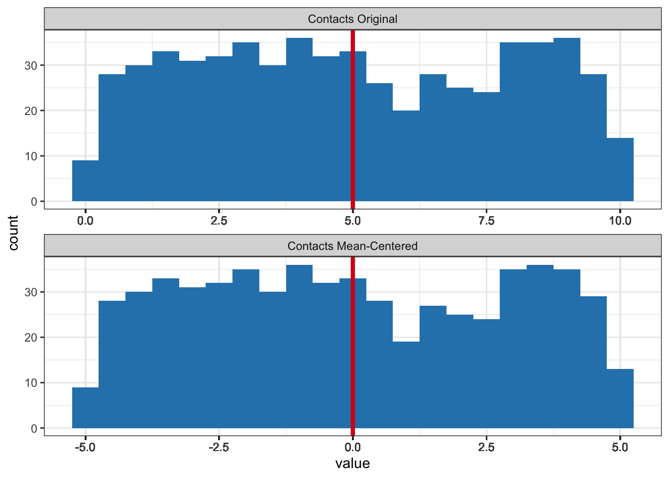
Figure 7.5: Histograms of the original contacts with smokers variable and the mean-centered variable. The red lines represent the means.
With mean-centered numerical moderators, a conditional effect in the presence of interaction always makes sense. It is the effect of the predictor for respondents who have an average score on the moderator because they score zero on the mean-centered variable. An average score always falls within the range of scores that actually occur. If we mean-center the moderator variable contact with smokers, the regression coefficient \(b_1\) for exposure expresses the effect of exposure on attitude for people with average contacts with smokers. This makes sense.
Remember that the interaction variable is the product of the predictor and moderator (Section 6.3.2). If any or both of these are mean-centered, you should multiply the mean-centered variable(s) to create the interaction variable.
7.1.4 Symmetry of predictor and moderator
If we want to interpret the conditional effect of contact on attitude (\(b_2\)), we must realize that this is the effect for people who score zero on the exposure variable if the exposure by contact interaction is included in the regression model. This is clear if we rearrange the regression equation as in Equation (7.3).
\[\begin{equation} \small \begin{split} attitude = &\ constant + b_1*exposure + b_2*contact + b_3*exposure*contact \\ attitude = &\ constant + b_1*exposure + (b_2 + b_3*exposure)*contact \\ attitude = &\ constant + b_1*0 + (b_2 + b_3*0)*contact \\ attitude = &\ constant + b_2*contact \end{split} \tag{7.3} \normalsize \end{equation}\]But wait a minute, this is what we would do if contact was the predictor and exposure the moderator. That is a completely different situation, is it not? No, technically it does not make a difference which variable is the predictor and which is the moderator (Figure 7.6). The predictor and moderator are symmetric. The difference is only in our theoretical expectations and in our interpretation.
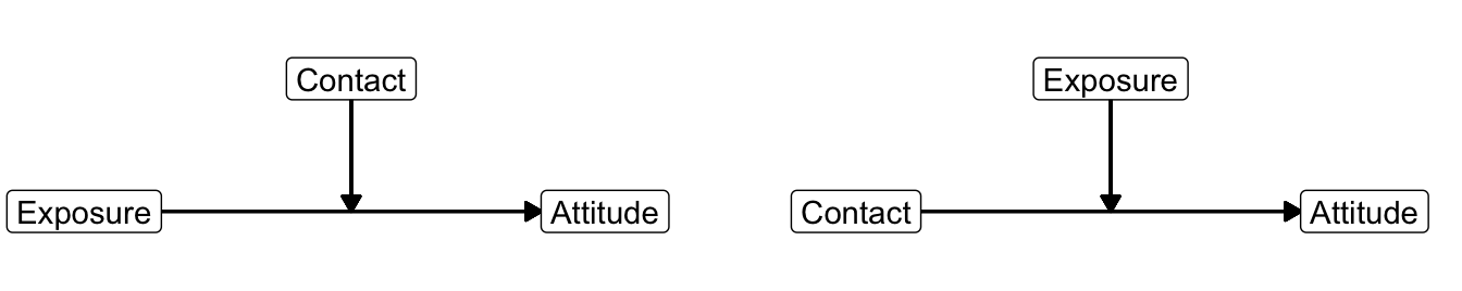
Figure 7.6: Two conceptual diagrams of moderation for the same interaction effect.
For example, let us assume that the regression coefficient of the interaction effect of exposure and contact is 0.2. We can interpret this regression coefficient with contact as moderator and exposure as predictor: An additional unit of contact with smokers increases the effect of exposure on attitude by 0.2. But we can also interpret it with exposure as moderator and contact as predictor: An additional unit of exposure increases the effect of contact with smokers on attitude by 0.2.
The conditional effect of the moderator, as stated above, is the effect of the moderator if the predictor is zero. This interpretation makes sense only if there are cases with zero scores on the predictor. In the current example, the scores on exposure range from 0 to 10, so zero exposure is meaningful. But it represents a borderline score with perhaps a very atypical effect of contact on attitude or few observations. For these reasons, it is recommended to mean-center both the predictor and moderator if they are numerical. In case of a dichotomous or categorical moderator (Section 6.3), the predictor can also be mean-centered.
7.1.5 Visualization of the interaction effect
It can be quite tricky to interpret regression coefficients in a regression model that contains interaction effects. The safest strategy is to draw regression lines for different values of the moderator. But what are interesting values if the moderator is numerical?
Figure 7.7: Which moderator values are helpful for visualizing moderation?
As we have seen in Section 7.1.1, the regression coefficient of an interaction effect with a numerical moderator can be directly interpreted. It represents the predicted difference in the unstandardized effect size for a one unit increase in the moderator. For example, one more contact with a smoker increases the exposure effect by 0.04.
The size of the interaction effect tells us the moderation trend, for instance, people who are more around smokers tend to be less opposed to smoking if they are exposed to the anti-smoking campaign. But we do not know how much an anti-smoking attitude is fostered by exposure to a campaign and whether exposure to the campaign increases anti-smoking attitude for everyone. Perhaps, people hanging out with smokers a lot may even get a more positive attitude towards smoking from campaign exposure.
We can be more specific about exposure effects at different levels of contact with smokers if we pick some interesting values of the moderator and calculate the conditional effects at these levels.
The minimum or maximum values of the moderator are usually not very interesting. We tend to have few observations for these values, so our confidence in the estimated effect at that level is low. Instead, the values one standard deviation below and above the mean of the moderator are popular values to be picked. One standard deviation below the mean (M - SD) indicates a low value, the mean (M) indicates a central value, and one standard deviation above the mean (M + SD) indicates a high value.
7.1.6 Statistical inference on conditional effects
| B | Std. Error | Beta | t | Sig. | Lower Bound | Upper Bound | |
|---|---|---|---|---|---|---|---|
| (Constant) | 0.169 | 0.204 | 0.825 | 0.412 | -0.238 | 0.575 | |
| Exposure (mean-centered) | -0.174 | 0.063 | -0.308 | -2.740 | 0.008 | -0.300 | -0.048 |
| Contact (mean-centered) | 0.159 | 0.094 | 0.188 | 1.685 | 0.096 | -0.029 | 0.347 |
| Status (smoker) | 0.533 | 0.405 | 0.131 | 1.318 | 0.191 | -0.272 | 1.338 |
| Exposure*Contact (mean-centered) | 0.018 | 0.034 | 0.063 | 0.533 | 0.595 | -0.049 | 0.085 |
The regression model yields a p value and confidence interval for the predictor at the reference value of the moderator. In the model estimated in Table 7.1, for instance, we obtain a p value of 0.008 and a 95% confidence interval of [-0.30, -0.05] for the effect of exposure on attitude. This is the conditional effect of exposure on attitude for cases that score zero on the moderator variable (contact with smokers).
If the moderator variable contact is mean-centered, the p value tests the null hypothesis that the effect of exposure is zero for people who have average contact with smokers. The confidence interval tells us that the effect of exposure on attitude for people with average contacts with smokers in the population ranges between -0.30 and -0.05 with 95% confidence. If the moderator is not mean-centered, the results apply to people who have no contact with smokers.
Note that mean-centering of the moderator changes, so to speak, the regression line that we test. Instead of testing the effect of exposure for people with no smoker contact, we test the effect for people with average contact with smokers if the moderator is mean-centered. If we would like to get the p value or confidence interval for the regression line at one standard deviation above (or below) the mean, we have to center the moderator at that value before we estimate the regression model. In this course, however, we will not do so.
7.1.7 Common support
In Section 6.3.6, we checked the support of the predictor in the data for different groups of the moderator. The basic idea is that we can only sensibly estimate and interpret a conditional effect at a moderator level if we have observations over the entire range of the predictor. For each moderator group, we checked the distribution of the predictor.
With a numerical moderator we can also do this if we group moderator scores. Hainmueller et al. (2016) recommend creating three groups, each containing one third of all observations. These low, medium, and high groups correspond more or less with the minus one standard deviation/mean/plus one standard deviation values that we used for visualizing and testing conditional effects. Create a histogram for the predictor in each of these groups to check common support of moderation in the data, as explained in micro lecture 6.26.
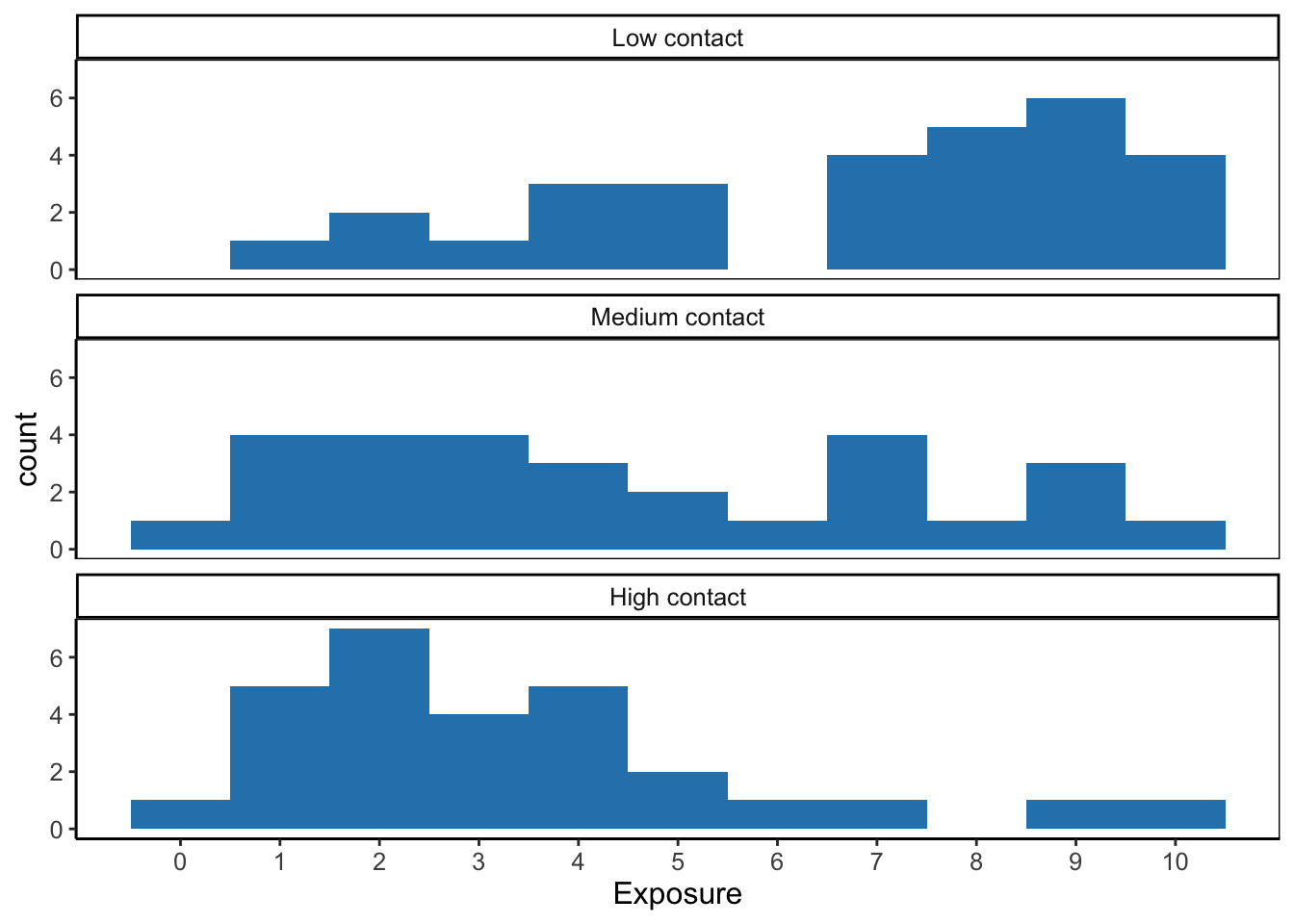
Figure 7.8: Common support of the predictor variable (exposure) at three levels of the moderator variable (contact).
According to Figure 7.8, the predictor variable exposure covers the entire range from 0 to 10 at medium and high contact levels. At low contact level, however, the lowest exposure score is 1 instead of zero. In all, we have common support for moderation of the exposure effect by contact for exposure scores from 1 to 10. This is quite a broad range but we should note that we have few observations of low exposure at the low contact level as well as few observations of high exposure at the high contact level.
7.1.8 Assumptions
The general assumptions for regression analysis (Section 6.1.4) also apply to a regression model with a moderator (interaction effect). The checks are the same: See if the residuals are more or less normally distributed and check the residuals by predicted values plot.
Note that the linearity assumption also applies to the interaction effect. If the interaction effect is positive, the exposure (predictor) effect must be higher for higher values of contact with smokers (moderator). More precisely, a unit difference on the moderator should result in a fixed increase (or decrease) of the effect of the predictor. You may have noticed this linear change in the effect size in Figure 7.3 at the beginning of this section on numerical moderators.
It is difficult to check this assumption, so let us not pursue this here. Just remember that the interaction effect is assumed to be linear: a gradually increasing or decreasing effect of the predictor at higher moderator values.
7.1.9 Higher-order interaction effects
An interaction effect with one moderator, whether numerical or categorical, is called first-order interaction or two-way interaction. It is possible to have a moderated effect that is moderated itself by a second moderator. For example, the change in the exposure effect due to a person’s contact with smokers may be different for smokers than for non-smokers. This is called a second-order interaction or three-way interaction. We can include more moderators, yielding even higher-order interactions, such as three or four moderators.
An interaction variable that is the product of the predictor and two moderators can be used to include a second-order interaction in a regression model. If you include a second-order interaction, you must also include the effects of the variables involved in the interaction as well as all first-order interactions among these variables in the regression model. All in all, these models become very complicated to interpret and they are beyond the scope of the current course.