5.4 Moderation: Group-Level Differences that Depend on Context
In the preceding section, we have analyzed the effects both of endorser and sex on willingness to donate to a fund raiser. The two main effects isolate the influence of endorser on willingness from the effect of sex and the other way around. This assumes that endorser and sex have an effect on their own, a general effect.
We should, however, wonder whether endorser always has the same effect. Even if there is a general effect of endorser on willingness to donate, is this effect the same for females and males? Note that one endorser is a male celebrity who is reputed to be quite attractive to women. The other endorser is a female celebrity with a similar reputation among men. In this situation, shouldn’t we expect that one endorser is more effective among female participants and the other among male participants?
If the effect of a factor is different for different groups on another factor, the first factor’s effect is moderated by the second factor. The phenomenon that effects are moderated is called moderation. Both factors are independent variables. To distinguish between them, we will henceforth refer to them as the predictor and the moderator.
With moderation, factors have a combined effect. The context (group score on one factor) affects the effect of the other factor on the dependent variable. The conceptual diagram for moderation expresses the effect of the moderator on the effect of the predictor as an arrow pointing at another arrow. Figure 5.11 shows the conceptual diagram for participant’s sex moderating the effect of endorsing celebrity on willingness to donate.
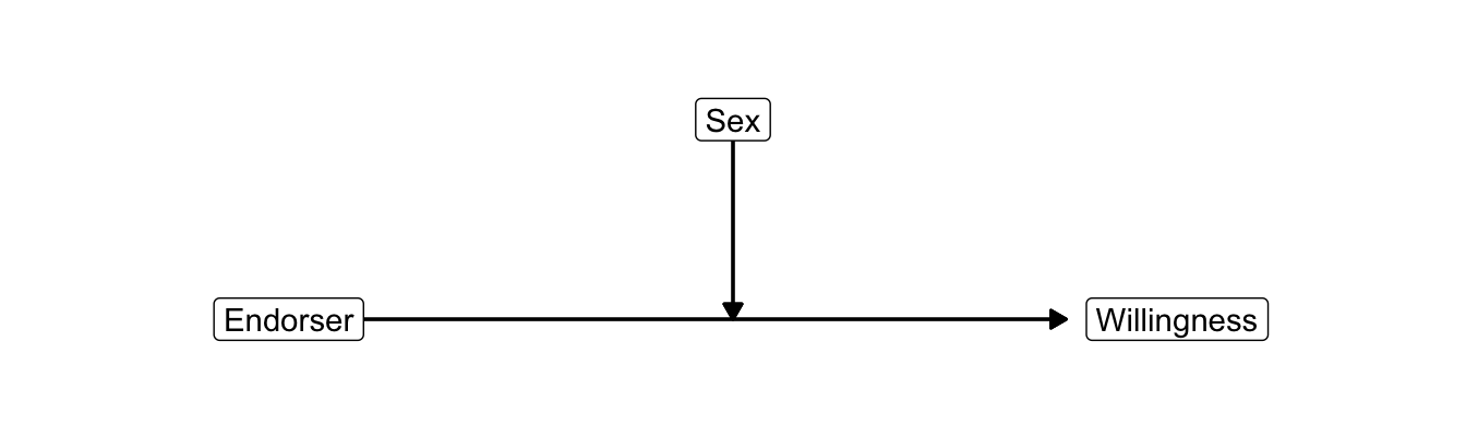
Figure 5.11: Conceptual diagram of moderation.
5.4.1 Types of moderation
Moderation as different effects for different groups is best interpreted using a cross-tabulation of group means, which is visualized as a means plot. In a group means table, the Totals row and column contain the means for each factor separately, for example the means for males and females (factor sex) or the means for the endorsers (factor endorser). These means represent the main effects. In contrast, the means in the cells of the table are the means of the subgroups, which represent moderation. Draw them in a means plot for easy interpretation.
In a means plot, we use the groups of the predictor on the horizontal axis, for example, the three endorsers. The average score on the dependent variable is used as the vertical axis. Finally, we plot the average scores for every predictor-moderator group, for instance, an endorser-sex combination, and we link the means that belong to the same moderator group, for example, the means for females and the means for males (Figure 5.12).
Figure 5.12: How can we recognize main effects and moderation in a means plot?
Moderation happens a lot in communication science for the simple reason that the effects of messages are stronger for people who are more susceptible to the message. If you know more people who have adopted a new product or a healthy/risky lifestyle, you are more likely to be persuaded by media campaigns to also adopt that product or lifestyle. If you are more impressionable in general, media messages are more effective.
5.4.1.1 Effect strength moderation
Moderation refers to contexts that strengthen or diminish the effect of, for instance, a media campaign. Let us refer to this type of moderation as effect strength moderation. In our current example, we would hypothesize that the effect of George Clooney as an endorser is stronger for female participants than for male participants.
In analysis of variance, effects are differences between average outcome scores. The effect of Clooney on willingness to donate, for instance, is the difference between the average willingness score of participants exposed to Clooney and the average score of participants who were not exposed to a celebrity endorser.
Different “Clooney effects” for female and male participants imply different differences! The difference in average willingness scores between females exposed to Clooney and females who are not exposed to an endorser is different from the difference in average scores for males. We have four subgroups with average willingness scores that we have to compare. We have six subgroups if we also include endorsement by Angelina Jolie.
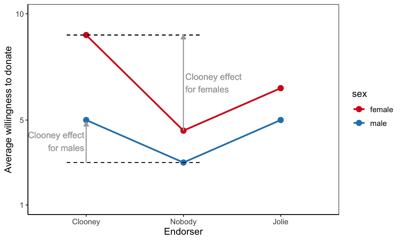
Figure 5.13: Moderation as a stronger effect within a particular context.
A means plot is a very convenient tool to interpret different differences. Connect the means of the subgroups by lines that belong to the same group on the factor you use as moderator. Each line in the plot represents the effect differences within one moderator group. If a line goes up or down, predictor groups have different means, so the predictor has an effect within that moderator group. A flat (horizontal) line tells us that there is no effect at all within that moderator group
The distances between the lines show the difference of the differences. If the lines for females and males are parallel, the difference between endorsers is the same for females and males. Then, the effects are the same and there is no moderation. In contrast, if the lines are not parallel but diverge or converge, the differences are different for females and males and there is moderation.
A special case of effect strength moderation is the situation in which the effect is absent (zero) in one context and present in another context. A trivial example would be the effect of an anti-smoking campaign on smoking frequency. For smokers (one context), smoking frequency may go down with campaign exposure and the campaign may have an effect. For non-smokers (another context), smoking frequency cannot go down and the campaign cannot have this effect.
Except for trivial cases such as the effect of anti-smoking campaigns on non-smokers, it does not make much sense to distinguish sharply between moderation in which the effect is strengthened and moderation in which the effect is present versus absent. In non-trivial cases, it is very rare that an effect is precisely zero. (See Holbert and Park (2019) for a different view on this matter.)
5.4.1.2 Effect direction moderation
In the other type of moderation, the effect in one group is the opposite of the effect in another group. In figure 5.14, for example, Clooney increases the average willingness to donate among females in comparison to the group who did not see a celebrity endorser. In contrast, average willingness for male Clooney viewers is lower than the average for males without endorser. Let us call this effect direction moderation. Males reverse the Clooney effect that we find for females.
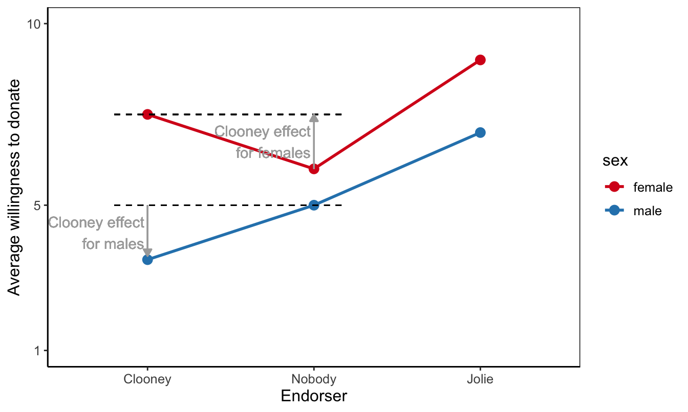
Figure 5.14: Moderation as a positive effect in one context and a negative effect in another context.
In an extreme situation, the effect in one group can compensate for the effect in another group if it is about as strong but of the opposite direction (Figure 5.15). Imagine that George Clooney convinces females to donate but discourages males to donate because his charms backfires on men (pure jealousy, perhaps.) Similarly, Angelina Jolie may have opposite effects on females and males.
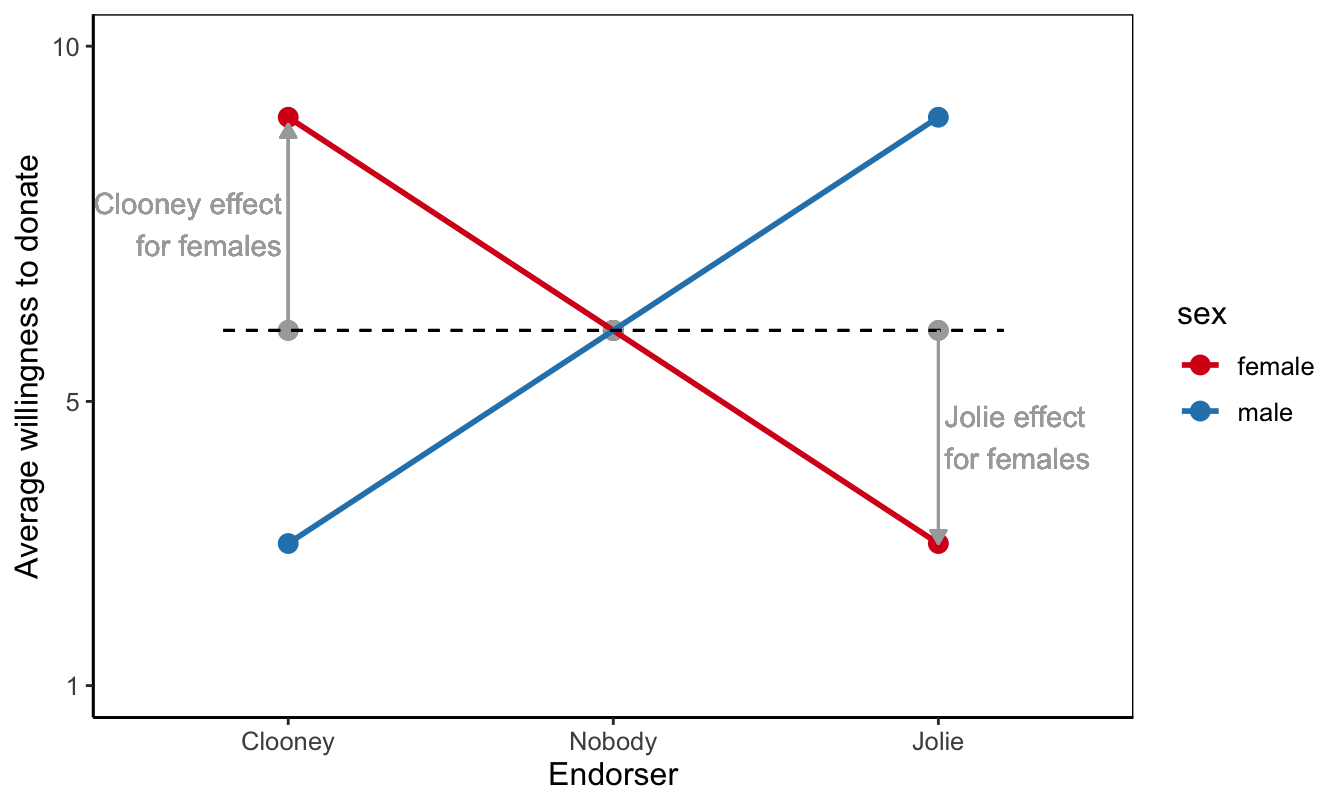
Figure 5.15: Moderation as opposite effects in different contexts.
In this situation, the main effect of endorser on willingness to donate is around zero. If we average over females and males, we obtain the means represented by the three grey dots. There is no net difference between Clooney, Jolie, and the condition without an endorser.
This does not mean that the endorser does not matter. On the contrary, the interaction effects tell us that the endorser is effective for one group but counterproductive for another group. The second part of the conclusion is just as important as the first part. The campaigner should avoid decreasing the willingness to donate among particular target groups.
5.4.2 Testing main and interaction effects
The effect of a single factor is called a main effect, as we learned in Section 5.3.3. A main effect reflects the difference between means for groups within one factor. The main effect of sex, for instance, can be that females are on average more willing to donate than males. A two-way analysis of variance includes two main effects, one for each factor (see Section 5.3.1), for example a main effect of sex and a main effect of endorser.
For moderation, however, we compare average scores of subgroups, that is, groups that combine a level on one factor with a level on another factor. In Figure 5.16, we compare average willingness to donate for combinations of endorser and participant’s sex. The effect of differences among subgroups on the dependent variable is called an interaction effect. Just like a main effect, an interaction effect is tested with an F test and its effect size is expressed by eta2.
Figure 5.16: How can we recognize main effects and moderation in a means plot?
Interpretation of moderation requires some training because we must look beyond main effects. The fact that females score on average higher than males is irrelevant to moderation but it does affect all subgroup mean scores. So the fact that the red line is above the blue line in Figure 5.16 is not relevant to moderation.
Moderation concerns the differences between subgroups that remain if we remove the overall differences between groups, that is, the differences that are captured by the main effects. The remaining differences between subgroup average scores provide us with a between-groups variance. In addition, the variation of outcome scores within subgroups yields a within-groups variance. Note that within-groups variance is not visible in Figure 5.16 because the willingness scores of the individual participants are not shown.
We can use the between-groups and within-groups variances to execute an F test just like the F test we use for main effects. The null hypothesis of the F test on an interaction effect states that the subgroups have the same population averages if we correct for the main effects. Our statistical software takes care of this correction if we include the main effects in the model, which we should always do.
Alternatively, we can formulate the null hypothesis of the test on the interaction effect as equal effects of the predictor for all moderator groups in the population. In the current example, the null hypothesis could be that the effect of endorser is the same for both sexes in the population. Or, the other way around, that the effect of sex is the same for different endorser groups in the population.
Moderation between three or more factors is possible. These are called higher-order interactions. It is wise to include all main effects and lower-order interactions if we test a higher-order interaction. As a result, our model becomes very complicated and hard to interpret. If a (first-order) interaction between two predictors must be interpreted as different differences, an interaction between three factors must be interpreted as different differences in differences. That’s difficult to imagine, so let us avoid them.
5.4.3 Assumptions for two-way analysis of variance
The assumptions for two-way analysis of variance are the same as for one-way analysis of variance (Section 5.1.4). Just note that equal group sizes and equal population variances now apply to the subgroups formed by the combination of the two factors.